Exploring the Operation of the Weaver Modulator for Single-Sideband Modulation

Compared to conventional amplitude modulation (AM), single-sideband (SSB) modulation offers significant savings in both bandwidth and power. In this series of articles, we’ve discussed three well-established methods for generating SSB signals. In order of their introduction, these are:

1. The filter method.
2. The phasing method.
3. Weaver’s method.

The previous article explained the basic principles of Weaver’s method using a single-frequency message signal. As we learned, the Weaver modulator requires neither the sharp bandpass filters used in the filter method nor the precise phase-shifters of the phasing method, making it the most practical of the three options listed above. Figure 1 shows the circuit diagram for the Weaver modulator.

 

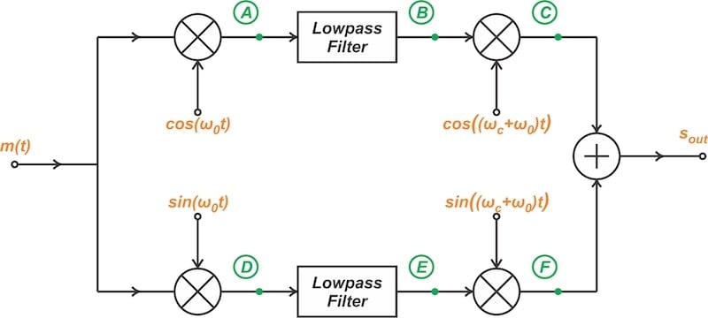
Figure 1. Weaver’s method for generating SSB signals.

 

In this article, we’ll continue our exploration of this circuit by examining how an arbitrary input spectrum changes as it passes through each of the six nodes—A through F—identified in the figure above. Nodes A through C represent the upper signal path; nodes D through C are located along the lower signal path. We’ll then examine the output spectrum created by combining the upper and lower path spectra.

Figure 2 shows our input spectrum, which has a bandwidth of B.

 

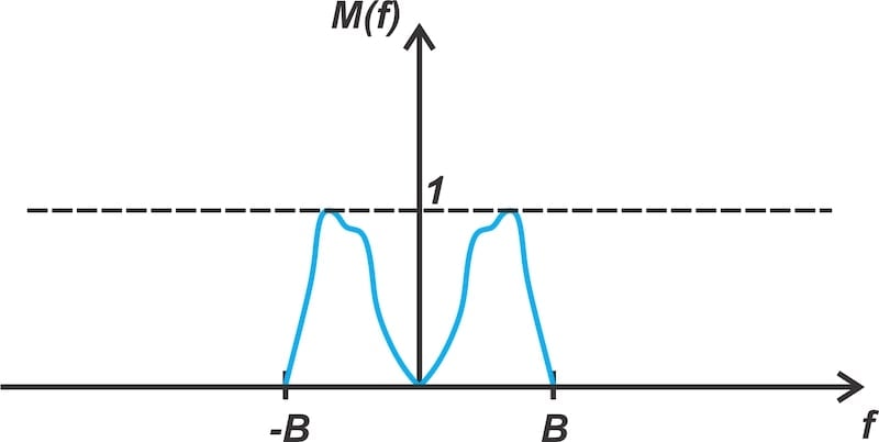
Figure 2. An example input spectrum for examining the Weaver modulator.

 

The Upper Path: Nodes A, B, and C

Let’s start by examining the upper path, which mixes the input with a cosine wave. Using Euler’s formula, the cosine term can be written as:

$$\cos( \omega_0 t) ~=~ \frac{1}{2} ( e^{j \omega_0 t} ~+~ e^{-j \omega_0 t} )$$

Equation 1.

 

In Weaver’s method, the first pair of multipliers mixes the message signal with an oscillator whose frequency (f₀) is in the center of the message signal’s frequency range. Since the message signal occupies a bandwidth of B, we have f₀ = B/2. The first multiplier therefore creates two signals: one with the spectrum shifted up in frequency by f₀, the other with the spectrum shifted down in frequency by the same amount. In both cases, the signal amplitude is halved.

Figure 3(b) shows the spectrum at the output of this multiplier (node A in the circuit diagram). To make the analysis easier to follow, the up- and down-shifted spectrum components are differentiated by color: green for downshifted, blue for upshifted.

 

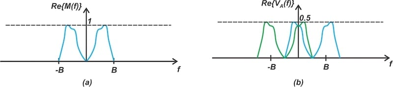
Figure 3. The signal spectrum at the input (a) and output (b) of the first multiplier on the upper path.

 

The vertical axes for both halves of Figure 3 are labeled as Re{.}, indicating that these spectrum components correspond to the real part of the signal spectrum. Unlike the mixers used in the lower path of the Weaver modulator, the mixing process that occurs between the input and node A doesn’t convert the real part of the input signal into an imaginary component.

From node A, the signal is then passed through a lowpass filter with a cutoff frequency of B/2. Figure 4 shows the spectrum at the filter’s output (node B).

 

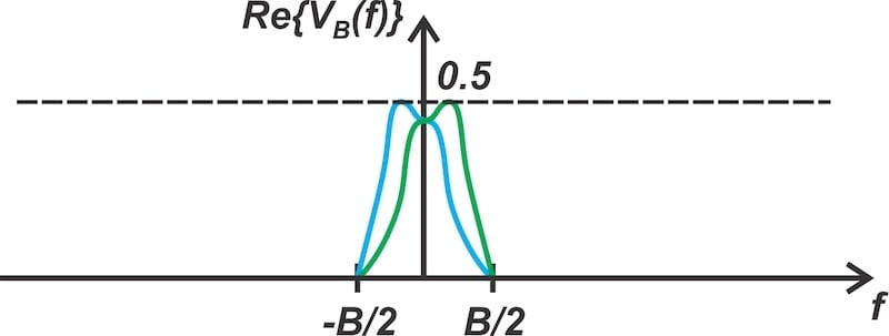
Figure 4. The signal spectrum at node B, divided into upshifted (blue) and downshifted (green) components.

 

The signal at the output of the lowpass filter is then fed into the second multiplier, where it’s mixed with a cosine wave of frequency f_c + f₀ = f_c + B/2.

Similar to what we saw in the first multiplier, the second multiplier of the upper path translates the spectrum by ±(f_c + B/2) and scales the amplitude by an additional factor of 0.5, resulting in an overall scaling factor of 0.25 with respect to the input spectrum.

Figure 5(d) shows the spectrum at the output of the second multiplier (node C).

 

Figure 5. The spectra at different nodes of the Weaver modulator’s upper path. [click to enlarge]

 

Taken as a whole, Figure 5 provides a summary of how the signal spectrum transforms as it travels from the input through the upper path.

 

The Lower Path: Nodes D, E, and F

In most ways, the functioning of the lower path is like that of the upper path. The difference is that it mixes the input with a sine wave, introducing a 90-degree phase shift. Using Euler’s formula, the sine function can be written as:

$$\sin( \omega_0 t) ~=~ \frac{1}{2j} ( e^{j \omega_0 t}~-~ e^{-j \omega_0 t} )$$

Equation 2.

 

The upshifted spectrum is multiplied by a factor of 1/(2j) = –0.5j, whereas the downshifted component experiences a scaling factor of –1/(2j) = 0.5j. The presence of the imaginary unit j means that the real part of the input spectrum is converted to an imaginary value at the output of the first multiplier (node D). The result is the spectrum shown in Figure 6(b).

 

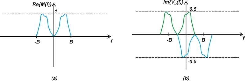
Figure 6. The spectra at the input (a) and node D (b) of the Weaver modulator.

 

Note that the vertical axis is changed from Re{.} to Im{.}, indicating that the figure shows the imaginary part of the spectrum.

Next, a lowpass filter with a cutoff frequency of B/2 eliminates all the frequency components outside of its passband. Figure 7 shows the spectrum at the filter’s output.

 

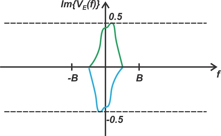
Figure 7. The spectrum at the output of the filter on the lower path (node E).

 

Finally, the second multiplier of the lower path translates the spectrum by ±(f_c + f₀) = ±(f_c + B/2). Due to multiplication by a sine function, the amplitudes of the upshifted and downshifted components are scaled by an additional factor of –0.5j and +0.5j, respectively.

However, the spectrum applied to the second multiplier (Figure 7), already has a scaling factor of j implied by the Im{.} notation next to the vertical axis. The upshifted and downshifted components are thus scaled by factors of –0.5j × j = 0.5 and +0.5j × j = –0.5, respectively. This means that the imaginary components are converted back into real components, as illustrated in Figure 8.

 

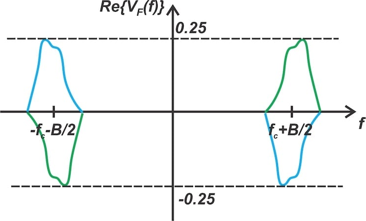
Figure 8. The spectrum at the output of the second multiplier on the lower path (node F).

 

Note that the vertical axis has changed from Im{.} to Re{.}, indicating that the figure shows the real part of the spectrum once again.

Figure 9 shows the spectra at all nodes of the lower path.

 

Figure 9. The frequency spectra from the beginning of the lower path to its end. [click to enlarge]

 

Determining the Output Spectrum

We obtain the output spectrum by combining the spectra of nodes C and F, which represent the respective outputs of the upper and lower paths. These spectra can be found in Figures 5(d) and 9(d). However, to help us more easily visualize this, Figure 10 also reproduces both spectra along with the final output spectrum.

 

Figure 10. The spectra at node C (top), node F (middle), and the modulator’s output (bottom). [click to enlarge]

 

As we can see, the upper sidebands emerge at the output. The lower sidebands are removed.

Figure 11 summarizes our analysis of the Weaver modulator. It displays the signal spectra at all nodes, including the circuit’s input and output.

 

Figure 11. The signal spectra at all nodes of Weaver’s modulator. [click to enlarge]

 

An Alternative Representation of the Lower Path Nodes

Some authors opt for a slightly different method of representing the spectrum components associated with the lower path. Instead of using Re{.} and Im{.} notations beside the vertical axis, they employ complex scaling factors for the various spectrum components. Figure 12 uses this approach to show the spectra of nodes D, E, and F within the lower path.

 

Figure 12. An alternative representation of the spectra at different nodes of the lower path. [click to enlarge]

 

For the sake of completeness, let’s briefly use the alternative representation to confirm our analysis.

Since the input, m(t), is mixed with a sine wave, the upshifted spectrum components in Figure 12(b) have a scaling factor of 1/2j. The downshifted spectrum components in Figure 12(b) experience a scaling factor of –1/2j. The lowpass filter eliminates the components above B/2 without changing the scaling factors, producing the spectrum in Figure 12(c).

Finally, the second mixer of the lower path multiplies the upshifted components in Figure 12(c) by 1/2j and the downshifted components by –1/2j. Since the green component in Figure 12(c) already has a scaling factor of –1/2j, its upshifted and downshifted replicas in Figure 12(d) have overall scaling factors of (–1/2j) × (1/2j) = 1/4 and (–1/2j) × (–1/2j) = –1/4, respectively.

Likewise, the blue component in Figure 12(c) already has a scaling factor of 1/2j. Therefore, the upshifted and downshifted replicas of this component will have overall scaling factors of (1/2j) × (1/2j) = –1/4 and (1/2j) × ( –1/2j) = 1/4. Comparing Figure 12(d) with Figure 11, we see that this result is consistent with our previous analysis.

 

Wrapping Up

In the previous article of this series, we described the basics of Weaver’s method by considering a single-frequency message signal and applying the concept of complex baseband representation. In this article, we used an arbitrary frequency spectrum to delve more deeply into the modulator’s operation. I hope that these discussions, taken together, have helped you develop a good working understanding of this useful SSB circuit.

This article also represents the final installment of a 15-part series on amplitude modulation in RF systems. A full list of articles in this series is provided below.

1. Introduction to Modulation Techniques in RF Systems
2. Understanding Double-Sideband Suppressed-Carrier Modulation
3. Understanding Conventional Amplitude Modulation
4. Understanding the Square-Law Modulator for Generating AM Signals
5. Introduction to the Balanced Modulator for AM Signals
6. How Do Switching Modulators Generate AM Signals?
7. Understanding How Ring Modulators Produce AM Signals
8. Four Interesting AM Modulation Circuits You Should Know About
9. Demodulating Double-Sideband AM Signals
10. Introduction to Single-Sideband Modulation: The Filter Method
11. The Phasing Method and Hilbert Transforms for Single-Sideband Modulation
12. A Visual Approach to Understanding the Phasing Method for SSB Modulation
13. How Phasors Help Us Understand Bandpass Signals
14. Introduction to Weaver’s Method for SSB Signal Generation
15. Exploring the Operation of the Weaver Modulator for Single-Sideband Modulation

 

All images used courtesy of Steve Arar