Introduction to Wideband FM Signals

Because it adheres to the superposition principle, amplitude modulation (AM) is classified as a linear modulation technique. Angle modulation, on the other hand, is fundamentally nonlinear. This nonlinearity complicates the analysis and design of both the transmitter and receiver systems.

One effect of this nonlinearity is that the effective bandwidth of the modulated wave can be much broader than that of the original message signal. To effectively transmit and receive angle-modulated signals, it’s essential to know the bandwidth that the modulated wave occupies.

Previously, we explored the frequency content of angle-modulated waves with a low modulation index. This article examines the bandwidth of angle-modulated waves with an arbitrary modulation index when the message signal is a single-frequency sinusoid. As before, we’ll focus on frequency modulation (FM) due to its superior noise performance.

 

Angle-Modulated Waves and Narrowband FM: A Review

To better grasp what we want to accomplish in this article, let’s start with a recap of what we covered in the previous ones. Recall that a constant-amplitude, angle-modulated signal can be represented by the following equation:

$$s(t) ~=~ A_c \cos( 2 \pi f_c t ~+~ \phi(t) )$$

Equation 1.

 

where A_c is the carrier amplitude and f_c is the carrier frequency.

Equation 2 shows the relationship between ϕ(t) and the message signal in FM schemes:

$$\phi (t) ~=~ 2 \pi k_f \int_{0}^{t} m(\tau) \ d \tau$$

Equation 2.

 

where k_f is the frequency deviation constant.

Though we won’t discuss phase modulation (PM) in this article, it also qualifies as angle modulation. For the sake of completeness, Equation 3 shows the relationship of ϕ(t) and the message signal in phase modulation:

$$\phi (t) ~=~ k_p m(t)$$

Equation 3.

 

where k_p is the proportionality constant.

Analyzing the bandwidth of angle modulation for an arbitrary message signal can quickly become very complex. For that reason, we often use certain approximations or special cases to understand the key characteristics of angle-modulated waves. One such approximation is narrowband angle modulation, which assumes that |ϕ(t)| is much less than one radian.

Our initial analysis found that narrowband FM occupies twice the bandwidth of the message signal. To further our understanding, we then considered narrowband FM modulation for the special case of a single-frequency message signal. This revealed that the lower sideband of narrowband FM experiences a phase reversal relative to the upper sideband, as depicted by the phasor diagram of Figure 1(b).

 

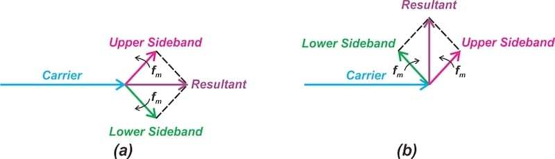
Figure 1. Phasor diagrams of conventional AM (a) and narrowband FM (b) when using a single-frequency message signal.

 

In this article, we’ll continue examining the bandwidth of FM waves created by a single-frequency message signal. Unlike in the previous article, however, the constraint of |ϕ(t)| ≪ 1 radian is lifted. We refer to this as wideband, as opposed to narrowband, FM.

 

Wideband FM With a Single-Frequency Input

Let’s assume that the message signal is a single-tone sinusoid:

$$m(t) ~=~ A_m \cos ( 2 \pi f_m t)$$

Equation 4.

 

where A_m and f_m are the message signal’s amplitude and frequency, respectively. Applying Equation 2, ϕ(t) for the FM wave is:

$$\phi(t) ~=~ \frac{k_f A_m}{ f_m} \sin( 2 \pi f_m t)$$

Equation 5.

 

The amplitude of ϕ(t), known as the modulation index, is commonly denoted by β:

$$\beta ~=~ \frac{k_f A_m}{ f_m} ~=~ \frac{ \Delta f}{f_m}$$

Equation 6.

 

where Δf = k_fA_m. Substituting Equation 5 into Equation 1, we obtain the FM signal:

$$s(t)~=~ A_c \cos \Big [ 2 \pi f_c t ~+~ \beta \sin(2 \pi f_m t) \Big ]$$

Equation 7.

 

The parameter β, which we introduced earlier as the modulation index, controls the amount of modulation in FM. As we’ll shortly see, the bandwidth of FM depends on β. Note that this is in contrast to the conventional AM scheme, whose bandwidth is independent of its modulation index (μ).

From Equation 6, β is directly proportional to the amplitude of the modulating signal (A_m) and inversely proportional to the modulating signal’s frequency (f_m). The bandwidth of FM therefore depends on both the amplitude and frequency of the modulating signal.

 

Determining the Occupied Bandwidth of an FM Wave

The FM wave produced by a sinusoidal modulating signal is generally non-periodic unless the carrier frequency (f_c) is an integral multiple of f_m. Nevertheless, it turns out that we can isolate a periodic multiplicative term from this equation. Using a Fourier series to expand this periodic term simplifies matters and allows us to identify the spectrum of the entire FM signal.

Let’s delve into this process. The FM signal in Equation 7 can be rewritten as:

$$s(t) ~=~ Re \big [ A_c e^{j \beta \sin(2 \pi f_m t)} e^{j 2 \pi f_c t} \big ]$$

Equation 8.

 

where the operator Re[.] denotes the real part of the quantity enclosed inside the square brackets. We define one of the multiplicative terms in Equation 8 as g(t):

$$g(t) ~=~ e^{j \beta \sin( 2 \pi f_m t)}$$

Equation 9.

 

This term is periodic, with a fundamental frequency equal to the modulation frequency. We can expand g(t) in the form of a complex Fourier series:

$$g(t) ~=~ \sum_{n=- \infty}^{\infty} c_n e^{j n \omega_m t}$$

Equation 10.

 

The exponential Fourier series coefficients of g(t) can be obtained as follows:

$$\begin{eqnarray}c_n &~=~& \frac{1}{T} \int_{-T/2}^{T/2} e^{j \beta \sin( \omega_m t)} e^{-j n \omega_m t} \ dt \\&~=~& \frac{1}{2 \pi} \int_{- \pi}^{\pi} e^{j \big ( \beta \sin(x) ~-~ nx \big )} \ dx \end{eqnarray}$$

Equation 11.

 

This integral, which is a function of both n and β, is known as the Bessel function of the first kind. It’s denoted by J_n(β):

$$\begin{eqnarray}c_n ~=~ J_n ( \beta) ~=~ \frac{1}{2 \pi} \int_{- \pi}^{\pi} e^{j \big ( \beta \sin(x) ~-~ nx \big )} \ dx \end{eqnarray}$$

Equation 12.

 

The above integral might seem daunting at first glance, but the good news is that we rarely need to compute it directly. We’ll delve into the key properties of J_n(β) in the next article. For now, just think of it as a scaling factor that’s dependent on n and β.

Having the Fourier series coefficients c_n = J_n(β), we can use Equation 10 to express g(t) as:

$$g(t) ~=~ \sum_{n=- \infty}^{\infty} J_n( \beta ) e^{j n \omega_m t}$$

Equation 13.

 

Finally, substituting this equation into Equation 8, the FM signal may be rewritten as:

$$s(t) ~=~ A_c \sum_{n ~ - \infty}^{n ~= \infty} J_n(\beta) \cos \big [( \omega_c ~+~ n \omega_m)t \big ]$$

Equation 14.

 

The above equation is a useful description of the FM signal with arbitrary modulation index β when the message signal is a single-frequency sinusoid.

 

Understanding the Derived Equation

Equation 14 shows that the carrier wave, scaled by a factor of J₀(β), appears in the output spectrum. The nearest components are the sidebands at f_c + f_m and f_c – f_m, which experience a scaling factor of J₁(β) and J_-1(β), respectively. The next closest components are the sidebands located at f_c + 2f_m and f_c – 2f_m, which respectively have scaling factors of J₂(β) and J_-2(β). This pattern continues for any J_n(β) and J_-n(β).

Figure 2 shows the typical spectrum of an FM signal generated by a sinusoidal modulating input for A_c = 1.

 

Figure 2. Typical spectrum of an FM signal for a single-tone message signal.

 

A few observations are in order here. First, in FM and PM, a large number of upper/lower sideband pairs are generated. This requires more bandwidth than amplitude modulation of the same message signal. Second, note that the frequency components are separated from one another by a frequency equal to the modulating frequency.

Finally, the amplitudes of the sidebands are not identical and are given by A_cJ_n(β). The scaling factor J_n(β) is a function of β, which is itself dependent on the amplitude (A_m) and frequency (f_m) of the message signal (see Equation 6). Therefore, the amplitudes of the frequency components change with A_m and f_m.

 

Example: Finding the FM Signal Spectrum

Now we’ll find the spectrum of the FM wave produced by a sinusoidal message signal for A_c = 1 and various modulation index values: β = 0, 0.2, 1, 2. To do this, we need to know the values of J_n(β).

To aid in determining the exact values of the Bessel functions, Table 1 lists J_n(β) for selected values of β. Values of J_n(β) below 0.01 are deemed negligible and thus are not included in the table.

 

Table 1. Significant values of J_n(β) for n = 0 through n = 14 and some selected values of β.

n	Jn(0.1)	Jn(0.2)	Jn(0.5)	Jn(1)	Jn(2)	Jn(5)	Jn(10)	n
0	1.00	0.99	0.94	0.77	0.22	–0.18	–0.25	0
1	0.05	0.10	0.24	0.44	0.58	–0.33	0.04	1
2			0.03	0.11	0.35	0.05	0.25	2
3				0.02	0.13	0.36	0.06	3
4					0.03	0.39	–0.22	4
5						0.26	–0.23	5
6						0.13	–0.01	6
7						0.05	0.22	7
8						0.02	0.32	8
9							0.29	9
10							0.21	10
11							0.12	11
12							0.06	12
13							0.03	13
14							0.01	14

 

Figure 3 shows J_n(β) for n = 0 through 4 and β ≤ 20.

 

Figure 3. Bessel functions of the first kind for n = 0 through 4 and β ≤ 20.

 

With β = 0, Figure 3 shows that we have J₀(0) = 1 and J_n(0) = 0 for all n > 0. In this case, we have no modulation. Only the unmodulated carrier, which has a relative amplitude of unity, appears at the output. This is illustrated in Figure 4(a).

 

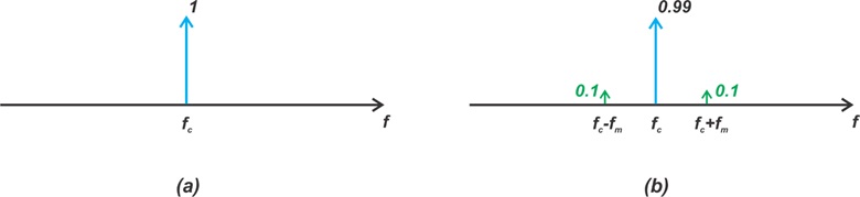
Figure 4. The magnitude of the FM signal spectrum for β = 0 (a) and β = 0.2 (b).

 

Figure 4(b) shows the magnitude of the output spectrum for β = 0.2. In Figure 4(b), the FM signal contains only a single pair of significant sidebands, similar to the conventional AM scheme. This is a case of narrowband FM, which we discussed in the previous article.

Finally, Figure 5(a) and Figure 5(b) show the output spectra obtained for β = 1 and β = 2, respectively.

 

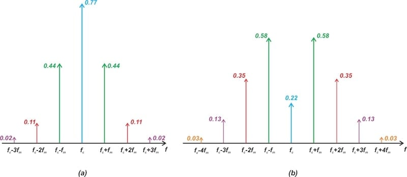
Figure 5. The magnitude of the FM signal spectrum for β = 1 (a) and β = 2 (b).

 

Comparing these plots to each other and to Figure 4, we see that increasing the modulation index results in additional significant sidebands. The amplitudes of the frequency components in Figures 4 and 5 match the corresponding values of Table 1.

 

Wrapping Up

The tone-modulated FM signal consists of a carrier component at f_c and an infinite number of sidebands at f_c ± f_m, f_c ± 2f_m, f_c ± 3f_m, and so on. The strength of the nth sideband is determined by the Bessel function, J_n(β). In the next article, we’ll take a closer look at the Bessel function so that we can better understand the behavior of the FM sidebands.

 

This article is Part 6 of a ten-part series on angle-modulated signals. All articles in this series are listed below in order of publication:

1. Introduction to Phase Modulation for RF Systems
2. Using Instantaneous Frequency to Represent PM and FM Signals
3. Understanding the Differences Between Phase and Frequency Modulation
4. Introduction to Narrowband Angle Modulation
5. Practical Insights Into Narrowband FM With a Single-Frequency Input
6. Introduction to Wideband FM Signals
7. Exploring Bessel Functions: Understanding the Spectrum of Tone-Modulated FM
8. Three Methods for Estimating the Transmission Bandwidth of FM Signals
9. Exploring the Relationship Between FM Wave Bandwidth and the Modulation Index
10. Estimating FM Wave Bandwidth: Solved Examples

 

All images used courtesy of Steve Arar