Using Instantaneous Frequency to Represent PM and FM Signals

Angle modulation techniques fall into two categories: phase modulation (PM) and frequency modulation (FM). The previous article in this series introduced phase modulation and provided several example waveforms to help us understand how the message signal influences the PM wave. Now, as we continue our discussion from a more mathematical perspective, we’ll expand our focus to include frequency modulation as well.

Using the concept of instantaneous frequency, we’ll create mathematical representations of both signal types. This, in turn, will help us explore the relationship between the two forms of angle modulation. As we’ll discover, PM and FM methods are so closely related that incorporating an additional circuit allows the modulator for one type to generate the other type’s signals.

 

PM Waves: The Relationship Between Phase and Frequency

An angle-modulated signal may be characterized as a sinusoidal function with a constant amplitude and an argument (θ_i) that varies according to the message signal being transmitted:

$$s(t) ~=~ A_c \cos[ \theta_i (t) ]$$

Equation 1.

 

We refer to θ_i as the instantaneous angle or instantaneous phase. In PM, the instantaneous angle varies linearly with the message signal, producing:

$$\theta_i (t)~=~2 \pi f_c t ~+~ k_p m(t)$$

Equation 2.

 

where:

f_c is the carrier frequency

k_p is the proportionality constant

m(t) is the message signal.

Figure 1 shows the PM wave generated by a sinusoidal message signal for a carrier frequency of f_c = 80 Hz and a constant value of k_p = 25 rad/V.

 

Figure 1. A sinusoidal message signal (top) and its corresponding PM wave (bottom).

 

As we see above, the descending part of the message waveform results in a decrease in the output frequency, whereas the ascending part increases the output frequency. The previous article provided several examples to demonstrate how the rising or falling portion of the message signal influences the PM wave’s frequency.

Another perspective on this phenomenon is that when the message signal increases over time, it adds an increasing term to the phase term contributed by 2πf_ct (see Equation 2). As a result, the phase of the modulated wave completes a full cycle more quickly. This shows up as an increase in frequency. Put another way, the PM wave compresses during the positive slope of m(t).

Conversely, when the message signal decreases over time, it contributes a negative phase change that counteracts part of the positive phase change caused by the 2πf_ct term. This means the modulated wave takes longer to complete a full cycle, resulting in a lower frequency. In other words, the PM waveform stretches during the negative slope of m(t).

To better understand this explanation, consider the following sinusoidal function for f_c = 100 Hz:

$$s(t) ~=~ \sin(2 \pi f_c t ~+~ \phi(t))$$

Equation 3.

 

where ϕ(t) is the added phase deviation. Figure 2 shows a quarter-period of this sinusoid for three distinct conditions of ϕ(t):

1. ϕ(t) = 0
2. ϕ(t) = 90 – 100t
3. ϕ(t) = 90 + 100t

 

Figure 2. One quarter-period of the wave described by Equation 3 for three different conditions of ϕ(t).

 

In the above figure, the blue curve (ϕ(t) = 0) represents an unmodulated wave. For the blue curve, one quarter of the period spans the interval from 0 to 2.5 ms.

The red curve (ϕ(t) = 90 + 100t) represents a PM wave where the message signal grows with time. In this case, the positive phase change from ϕ(t) adds to that from the 2πf_ct term. Consequently, more than one quarter of the period fits within the 0 to 2.5 ms interval.

Finally, the green curve (ϕ(t) = 90 – 100t) represents a PM wave with a decreasing phase term. The negative phase change from ϕ(t) offsets part of the positive phase change from the 2πf_ct term. As a result, less than one quarter of the waveform fits within the 0 to 2.5 ms interval.

 

Instantaneous Frequency

An unmodulated signal with frequency f_c, amplitude A_c, and initial phase ϕ₀ can be represented by a phasor that rotates at a constant angular velocity of 2πf_c. This is shown in Figure 3(a). An angle-modulated signal acts as a phasor with amplitude A_c that rotates at a time-dependent angular velocity, as illustrated in Figure 3(b).

 

Figure 3. Phasor representation of an unmodulated signal (a) and an angle-modulated signal (b).

 

Let’s take a closer look at the angle-modulated wave. How can we characterize its frequency of rotation? When θ_i changes by 2π radians, the corresponding phasor completes a full cycle of rotation. Therefore, the average frequency in hertz over an interval from t to (t + Δt) can be obtained by:

$$f_{ave} ~=~ \frac{ \theta_i (t~+~ \Delta t) ~-~ \theta_i (t)}{2 \pi \Delta t}$$

Equation 4.

 

In the special case of an unmodulated carrier wave with frequency f_c and initial phase ϕ₀, the above equation produces:

$$f_{ave} ~=~ \frac{ [2 \pi f_c (t~+~ \Delta t) ~+~ \phi_0 ] ~-~ [2 \pi f_c t ~+~ \phi_0 ]}{2 \pi \Delta t}~=~f_c$$

Equation 5.

 

As this demonstrates, the average frequency for an unmodulated carrier wave is equal to f_c. For an angle-modulated signal, the average frequency depends on the value of the message signal over the time interval of interest. However, if we let Δt in Equation 4 approach zero, the obtained frequency can be interpreted as the instantaneous frequency, f_i(t), of the rotating phasor. For Δt → 0, the equation can be rewritten in terms of the time derivative of θ_i:

$$f_i(t) ~=~ \frac{1}{2 \pi} \frac{d \theta_i}{dt}$$

Equation 6.

 

Using the above equation, the angular velocity of the corresponding phasor is equal to 2πf_i(t) rad/s.

By applying the concept of instantaneous frequency, we can explain the behavior of the PM wave in Figure 1. If we substitute θ_i from Equation 2 into the instantaneous frequency equation, we obtain:

$$\begin{eqnarray}f_i(t) &~=~& \frac{1}{2 \pi} \frac{d \theta_i}{dt} \\&~=~&\frac{1}{2 \pi} \frac{d }{dt} \big [ 2 \pi f_c t ~+~ k_p m(t) \big ] \\&~=~& f_c ~+~ \frac{k_p}{2 \pi} \frac{dm(t) }{dt} \end{eqnarray}$$

Equation 7.

 

This implies that as the message signal increases over time, the output frequency rises. Conversely, as the message signal decreases, the output frequency drops.

 

Representing PM and FM Signals

Now that we understand the basics of both instantaneous phase and instantaneous frequency, we can use them to provide a unified description of PM and FM schemes. By writing the instantaneous phase as:

$$\theta_i(t) ~=~ 2 \pi f_c t ~+~ \phi(t)$$

Equation 8.

 

where ϕ(t) is the phase deviation, we can express the angle-modulated wave described by Equation 1 as follows:

$$s(t) ~=~ A_c \cos( 2 \pi f_c t ~+~ \phi(t) )$$

Equation 9.

 

This shows that the instantaneous phase is the sum of a central value set by the terms 2πf_ct and ϕ(t). In both forms of angle modulation, ϕ(t) depends on the message signal. For PM, ϕ(t) is directly proportional to the message signal:

$$\phi (t) ~=~ k_p m(t)$$

Equation 10.

 

where k_p is the proportionality constant. Assuming that m(t) is a voltage quantity, k_p is expressed in radians per volt.

The instantaneous frequency of the modulated wave described by Equation 9 is determined by taking the derivative of the instantaneous phase:

 

$$f_i(t) ~=~ \frac{1}{2 \pi} \frac{d \theta_i}{dt} ~=~ f_c ~+~ \frac{1}{2 \pi} \frac{d \phi}{dt}$$

Equation 11.

 

The message-dependent part of the instantaneous frequency is called the frequency deviation:

$$frequency~~deviation ~=~ \frac{1}{2 \pi} \frac{d \phi}{dt}$$

Equation 12.

 

In an FM system, the frequency deviation is proportional to the message signal:

$$\frac{1}{2 \pi} \frac{d \phi}{dt} ~=~ k_f m(t)$$

Equation 13.

 

where k_f is the frequency deviation constant. Assuming that m(t) is a voltage quantity, k_f is expressed in hertz per volt.

Taking the integral of the above equation, we can determine ϕ(t) and substitute it in Equation 8 to arrive at the FM signal equation:

$$s_{FM}(t) ~=~ A_c \cos \big [ 2 \pi f_c t ~+~ 2 \pi k_f \int_{0}^{t} m(\alpha) d \alpha \big ]$$

Equation 14.

 

Note that a constant would normally appear in the above equation due to integration. However, we’re assuming that the unmodulated wave’s angle is zero at t = 0. This eliminates the constant.

While we're on the subject of constants, it's worth mentioning that the proportionality constant (k_p) has several different names. Depending on which reference you consult, you may find k_p described as the phase deviation constant, the phase sensitivity of the modulator, the phase modulation index, or simply as the modulation index. Similarly, k_f—the frequency deviation constant—is sometimes called the frequency sensitivity of the modulator.

 

The Relationship Between FM and PM

FM and PM modulators can produce identical outputs if we establish a specific relationship between their inputs. To understand this, consider Equation 14 alongside the PM signal equation reproduced below:

$$s_{PM}(t) ~=~ A_c \cos[ 2 \pi f_c t ~+~ k_p m(t) ]$$

Equation 15.

 

From Equations 14 and 15, the following relationship is required for the two methods to produce the same output:

$$k_p m_p(t) ~=~ 2 \pi k_f \int_{- \infty}^{t} m_f(\alpha) d \alpha$$

Equation 16.

 

where:

m_f(t) is the input applied to the FM modulator

m_p(t) is the input applied to the PM modulator.

From Equation 16, we see that the PM and FM circuits produce identical outputs if m_p(t) is the integral of m_f(t). In short, if we place an integrator at the input of a phase modulator, we can use it to produce FM signals. This setup is illustrated in Figure 4.

 

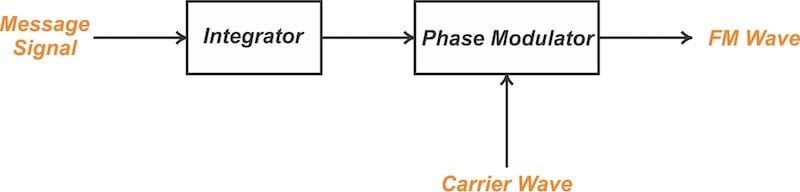
Figure 4. Using a phase modulator to generate FM waves.

 

Equation 16 also shows that the two types of modulator produce the same output if the signal applied to the FM modulator is equal to the derivative of the signal applied to the PM modulator. This implies that an FM modulator can be used to generate PM signals if we differentiate the message signal before using it as the input to the FM modulator (Figure 5).

 

Figure 5. Generating PM waves by using an FM modulator.

 

Consider, for example, the square wave message m(t) illustrated in the top left portion of Figure 6.

 

Figure 6. Top left: A square-wave message signal. Bottom left: its corresponding FM wave. Top right: an unmodulated sawtooth wave. Bottom right: its corresponding PM wave.

 

The FM wave corresponding to the square-wave message is shown (f_c = 5 Hz, k_f = 1.59 Hz/V) in the lower left quadrant of this figure. The upper right quadrant of the figure shows a sawtooth wave; the lower right quadrant displays its PM wave for k_p = 10 rad/V.

Placed side by side, the two modulated waves appear identical. Since the integral of a square wave results in a sawtooth signal, this isn’t surprising.

 

Wrapping Up

In this article, we advanced our understanding of angle modulation—both PM and FM—by incorporating a mathematical perspective. We delved into the concept of instantaneous frequency and, using that concept, examined the close relationship between PM and FM methods. I hope this article has helped you gain a deeper appreciation of these modulation methods and the time-domain behavior of the signals they produce.

 

This article is Part 2 in a ten-part series on angle-modulated signals. All articles in this series are listed below in order of publication:

1. Introduction to Phase Modulation for RF Systems
2. Using Instantaneous Frequency to Represent PM and FM Signals
3. Understanding the Differences Between Phase and Frequency Modulation
4. Introduction to Narrowband Angle Modulation
5. Practical Insights Into Narrowband FM With a Single-Frequency Input
6. Introduction to Wideband FM Signals
7. Exploring Bessel Functions: Understanding the Spectrum of Tone-Modulated FM
8. Three Methods for Estimating the Transmission Bandwidth of FM Signals
9. Exploring the Relationship Between FM Wave Bandwidth and the Modulation Index
10. Estimating FM Wave Bandwidth: Solved Examples

 

Featured image used courtesy of Adobe Stock; all other images used courtesy of Steve Arar