Estimating FM Bandwidth: Solved Examples

In this article, we'll illustrate the usefulness of Carson's rule for bandwidth estimation by working through a series of example problems.

Technical Article August 10, 2025 by Dr. Steve Arar

Earlier articles in this series explored the principles of FM wave bandwidth. In this article, we'll solidify those concepts by walking through several detailed examples of FM wave bandwidth calculations using Carson's rule. As we know from our earlier discussion, this is a convenient way to determine an FM signal's effective bandwidth.

Carson's rule is given by:

$$BW ~=~ 2(\Delta f ~+~ f_m)~=~ 2(\beta ~+~ 1)f_m$$

Equation 1.

where:

Δf is the frequency deviation

f_m is the modulating frequency

β is the modulation index.

With that, let's jump straight into the examples!

Example 1: Bandwidth of a Tone-Modulated Wave

As our first example, let's estimate the transmission bandwidth of the following FM signal:

$$s(t) ~=~ 10 \cos \big [ 90 ~\times~ 10^6 t ~+~ 200 \cos (2000t) \big ]$$

Equation 2.

Solution to Example 1

To solve this problem using Carson's rule, we need to know the values of Δf and f_m for the above signal. Recall that the general form of a tone-modulated FM wave is given by:

$$s(t)~=~ A_c \cos \Big [ 2 \pi f_c t ~+~ \beta \sin(2 \pi f_m t) \Big ]$$

Equation 3.

where A_c is the amplitude of the carrier signal and f_c is its frequency.

Comparing this equation to Equation 2, we see that f_m is:

$$f_m ~=~ \frac{2000}{2\pi}~=~318.31 \ \text{Hz}$$

Equation 4.

Next, we need to find the frequency deviation (Δf). To do so, we first need to determine the instantaneous frequency. The instantaneous frequency is the derivative of the sinusoid's argument:

$$ \begin{eqnarray} \omega_i &~=~& \frac{d}{dt} \big [ 90 ~\times~ 10^6 t ~+~ 200 \cos (2000t) \big ] \\ &~=~& 90 ~\times~ 10^6 ~-~ 4 ~\times~ 10^5 \sin(2000t) \end{eqnarray} $$

Equation 5.

From this, the frequency deviation in Hz is found to be:

$$\Delta f ~=~ \frac{1}{2 \pi} ~\times~ 4 ~\times~ 10^5 ~=~ 63.66 \ \text{kHz}$$

Equation 6.

We now know both the modulating frequency (f_m = 318.31 Hz) and the frequency deviation (Δf = 63.66 kHz). Substituting these values into Carson's equation, we find the approximate bandwidth:

$$BW ~=~ 2(\Delta f ~+~ f_m)~=~2(63.66 \ \text{kHz} ~+~ 318.31 \ \text{Hz})~=~ 127.96 \ \text{kHz}$$

Equation 7.

Alternatively, we can determine the modulation index (β) the same way we did f_m. This method achieves the same result without requiring us to calculate the frequency deviation.

Comparing Equations 2 and 3, we obtain β = 200. We then apply the second form of Carson's rule:

$$BW ~=~2(\beta ~+~ 1)f_m ~=~ 2(200~+~1) ~\times~ 318.31 ~=~ 127.96 \ \text{kHz}$$

Equation 8.

Example 2: Interpreting an Angle-Modulated Wave as an FM or PM Wave

Let's take another look at the signal from Equation 2. For convenience, it's reproduced below:

$$s(t) ~=~ 10 \cos \big [ 90 ~\times~ 10^6 t ~+~ 200 \cos (2000t) \big ]$$

Equation 9.

Though we previously referred to it as an FM signal, the angle-modulated wave in Equation 9 could be either phase-modulated (PM) or frequency-modulated (FM). In either case, we can apply Carson's rule to find the bandwidth. However, changing the modulating signal's frequency affects the spectra of PM and FM signals differently.

If we assume s(t) is a PM wave, how does its bandwidth change with f_m? What about if it's an FM wave? Let's find out!

Example 2 as a PM Wave

The PM wave generated by a single-frequency message signal, m(t) = A_mpcos(2πf_mt)), can also be described by the following equation:

$$s(t) ~=~ A_c \cos \big [2 \pi f_c t ~+~ k_p m(t) \big ]~=~ A_c \cos \big [2 \pi f_c t ~+~ k_p A_{mp} \cos( 2 \pi f_m t) \big ]$$

Equation 10.

where k_p is the phase deviation constant.

Comparing Equation 10 with the general form of the signal in Equation 3, we see that β is equal to k_pA_mp and is independent of f_m. Using Carson's equation, the bandwidth is given by:

$$BW ~=~ 2(\beta ~+~ 1)f_m$$

Equation 11.

Because it's independent of f_m, β remains constant. The bandwidth is therefore directly proportional to f_m. For example, we currently have a modulation index of β = 200 and a modulating frequency of f_m = 318.31 Hz. If we increase the modulating frequency by a factor of two, the bandwidth of the PM signal also doubles from 127.96 kHz to 255.92 kHz.

Next, let's interpret s(t) as an FM wave.

Example 2 as an FM Wave

For a tone-modulated FM signal, it can be easily shown that the modulation index is given by:

$$\beta ~=~ \frac{k_f A_m}{ f_m} ~=~ \frac{ \Delta f}{f_m}$$

Equation 12.

Note that β is inversely proportional to f_m. If we double f_m from 318.31 Hz to 636.62 Hz, the modulation index is halved from 200 to 100. Applying Carson's rule, the bandwidth is:

$$BW ~=~ 2(\beta ~+~ 1)f_m ~=~ 2(100~+~1) ~\times~ 636.62 ~\approx~ 128.6 \ \text{kHz}$$

Equation 13.

Unlike the PM wave, the bandwidth of the FM wave changes only slightly with the modulating frequency.

Example 3: FM Wave Produced by a Two-Tone Message Signal

Consider a message signal that consists of two sinusoids:

$$m(t) ~=~ A_1 \cos(2 \pi f_1 t) ~+~ A_2 \cos(2 \pi f_2 t)$$

Equation 14.

This leads to an FM wave in the form of:

$$s(t) ~=~ A_c \cos \big [2 \pi f_c t ~+~ \beta_1 \sin(2 \pi f_1 t) ~+~ \beta_2 \sin(2 \pi f_2 t) \big ]$$

Equation 15.

Let's use Carson's rule to estimate the bandwidth of s(t) for the following parameter values:

β₁ = β₂ = 5
f_c = 5 kHz
f₁ = 2 Hz
f₂ = 53 Hz.

Solution to Example 3

As in Example 1, we need to determine the instantaneous frequency (⍵_i) in order to find the frequency deviation (Δf). Taking the derivative of the sinusoid's argument, we obtain:

$$\omega_i ~=~ 2 \pi f_c ~+~ \beta_1 ~\times~ 2 \pi f_1 ~\times~ \cos(2 \pi f_1 t) ~+~ \beta_2 ~\times~ 2 \pi f_2 ~\times~ \cos(2 \pi f_2 t)$$

Equation 16.

Hence, Δf in Hz is found to be:

$$\begin{eqnarray} \Delta f &~=~& Maximum \ of \ \Big [ \beta_1 ~\times~ f_1 ~\times~ \cos(2 \pi f_1 t) ~+~ \beta_2 ~\times~ f_2 ~\times~ \cos(2 \pi f_2 t) \Big ] \\ &~=~& \beta_1 ~\times~ f_1 ~+~ \beta_2 ~\times~ f_2 \\ &~=~& 5 ~\times~ 2 ~+~ 5 ~\times~ 53 \\ &~=~& 275 \ \text{Hz} \end{eqnarray}$$

Equation 17.

Note that the two cosine terms inside the square brackets become in-phase at some points (at t = 0, for example). The maximum value is thus equal to the sum of the amplitudes of the individual cosine waves.

To find the signal bandwidth, we replace f_m in Carson's equation with the highest frequency contained in the message signal (W). Noting that W = 53 Hz in this case, we have:

$$BW ~=~ 2 (\Delta f ~+~ W) ~=~ 2 (275 ~+~ 53) ~=~ 656 \ \text{Hz}$$

Equation 18.

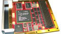
Figure 1 illustrates the output spectrum near the carrier frequency (f_c = 5 kHz). The spectrum was obtained by performing an FFT on the modulated signal.

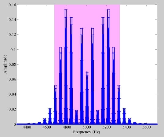
The spectrum of the FM wave near the carrier frequency.

Figure 1. The spectrum of the FM wave near the carrier frequency (f_c = 5 kHz).

The shaded magenta region in this figure represents the bandwidth obtained from Carson's rule, which ranges from 4,672 Hz to 5,328 Hz. While Carson's rule provides a good estimate of the signal bandwidth, we see above that it may somewhat understate the bandwidth of a practical FM system.

Note that when the message signal consists of two tones at f₁ and f₂, the FM signal comprises frequency components at f_c + nf₁ and f_c + mf₂, as well as at f_c + nf₁ + mf₂, for all possible values of n and m. This is illustrated in Figure 2, which provides a close-up of Figure 1 around the carrier frequency.

A close-up view of the FM wave's spectrum near the carrier frequency.

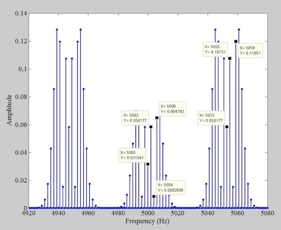
Figure 2. A close-up view of the FM wave's spectrum near the carrier frequency.

The figure displays the frequency and amplitude of various frequency components, providing clarity on the frequencies at which the sidebands appear. For instance, we have sidebands at:

f_c + f₁ = 5,002 Hz, f_c + 2f₁ = 5,004 Hz, …
f_c + f₂ = 5,053 Hz, f_c + 2f₂ = 5,106 Hz, …
f_c + f₁ + f₂ = 5,055 Hz, f_c + 2f₁ + f₂ = 5,057 Hz, …
f_c + f₁ + f₂ = 5,055 Hz, f_c + f₁ + 2f₂ = 5,108 Hz, …

For a double-tone message signal comprising a high frequency component (f₂) and a low frequency component (f₁), we observe an interesting property—namely, that the sideband components around f_c + mf₂ resemble an FM wave with carrier frequency of f_c + mf₂ and modulating frequency of f₁.

Example 4: FM Wave Produced by a Triangular Wave

For our final example, we'll consider a periodic, triangular message signal that ramps up from –1 to 1 and then back to –1. As shown in Figure 3, it repeats itself with a period of 2 ms.

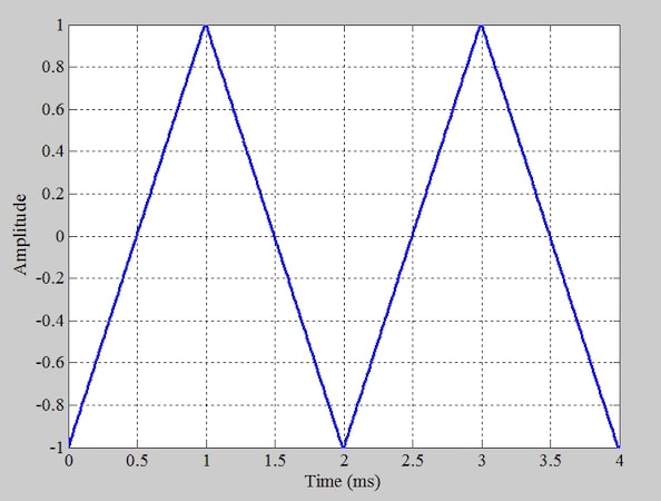
The periodic triangle wave we'll use to generate an FM signal.

Figure 3. The periodic triangle wave we'll use to generate an FM signal.

Estimate the bandwidth of the FM wave produced by the above message signal if the frequency deviation constant(k_f) is 5 kHz/V and the carrier frequency is f_c = 25 kHz.

Solution to Example 4

For arbitrary m(t), we can apply Carson's rule written in terms of the deviation ratio (D) to estimate the bandwidth:

$$BW ~=~ 2 (\Delta f ~+~ W) ~=~ 2(D~+~1)W$$

Equation 19.

where W is the highest frequency contained in the message signal.

The deviation ratio is given by:

$$D ~=~ \frac{k_f}{W} ~\times~ Max(|m(t)|)$$

Equation 20.

To determine W, we'll examine the spectrum of the triangle-wave message signal in Figure 3. This spectrum is shown in Figure 4.

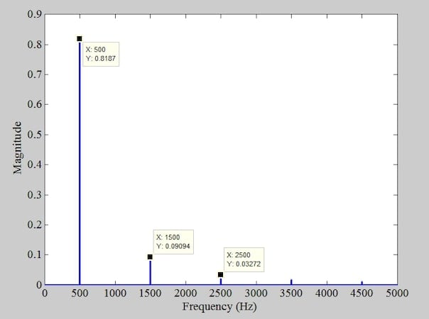
The single-sided spectrum of the message signal.

Figure 4. The single-sided spectrum of the message signal.

The fundamental frequency is 500 Hz, with higher harmonics dropping off rapidly. For example, the fifth harmonic at 2,500 Hz has an amplitude that's just 4% of the fundamental, resulting in a power that's only 0.16% of the fundamental power.

Let's assume that the third harmonic is the highest significant frequency component of the signal (W = 1,500 Hz). Noting that the maximum value of m(t) is unity, Equation 20 produces:

$$D ~=~ \frac{k_f}{W} ~\times~ Max(|m(t)|) ~=~ \frac{5000}{1500} ~\times~ 1~=~ 3.33$$

Equation 21.

This leads to an estimated bandwidth of:

$$BW~=~2(D~+~1)W~=~2(3.33~+~1)~\times~1500~=~12.99 \ \text{kHz}$$

Equation 22.

Figure 5 shows the spectrum of the modulated signal around the carrier frequency (f_c = 25 kHz).

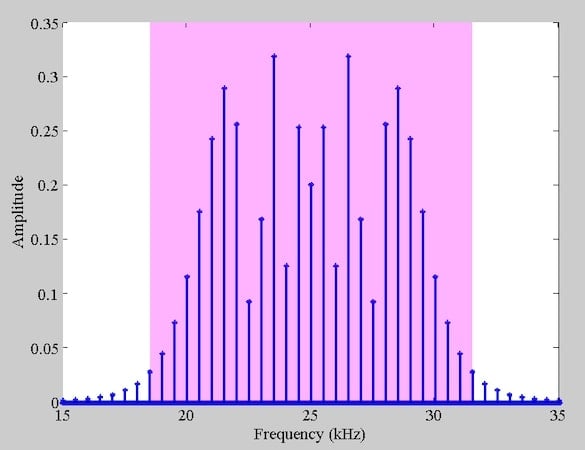
The spectrum of the FM wave near the carrier frequency.

Figure 5. The spectrum of the FM wave near the carrier frequency (f_c = 25 kHz).

In the above figure, the shaded magenta region once again represents the bandwidth obtained from Carson's rule. It's evident that Carson's rule effectively estimates the signal bandwidth in this case.

Wrapping Up

In this article, we examined four different bandwidth calculation examples using Carson's rule. This useful approximation captures most (at least 98%) of the significant sideband energy of the FM wave, making it a practical tool for spectrum planning and analysis.

As we finish up here, it's important to note that most of our discussion in this article series has centered on tone-modulated FM waves. Real-world message signals are far more complex. Although examining the single-tone case can offer valuable insights into certain properties of FM waves, generalizing these findings can sometimes be misleading. For instance, FM delivers an output SNR three times higher than PM with a single-tone input, but this doesn't apply to most practical signals.

This article is the final installment in a ten-part series on angle-modulated signals. All articles in this series are listed below in order of publication: