Exploring the Relationship Between FM Wave Bandwidth and the Modulation Index

Earlier in this series, we examined the spectrum of FM waves produced by a single-frequency message signal. In this article, we'll continue our discussion by analyzing the effects of the modulating signal's frequency and amplitude on the spectrum of a tone-modulated FM wave. Towards the end of the article, we'll also look at how the modulation index parameters in AM and FM differ from each other.

 

The Spectrum of Tone-Modulated FM

Figure 1 shows the typical spectrum of a tone-modulated FM wave when the carrier wave has an amplitude of unity.

 

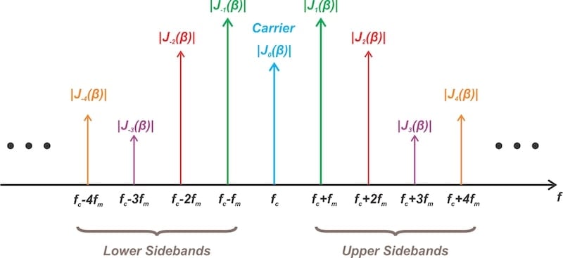
Figure 1. Typical spectrum of an FM signal for a single-tone message signal.

 

The spectrum includes distinct tones separated by the modulating frequency (f_m). These tones are found at the carrier frequency (f_c) and sideband frequencies f_c ± f_m, f_c ± 2f_m, f_c ± 3f_m, and so on. The amplitude of the nth sideband is scaled by the Bessel function of the first kind, J_n(β), where β represents the modulation index.

The modulation index is given by:

$$\beta ~=~ \frac{k_f A_m}{ f_m} ~=~ \frac{ \Delta f}{f_m}$$

Equation 1.

 

where:

A_m is the amplitude of the modulating signal

k_f is the frequency deviation constant

Δf is the maximum frequency deviation.

In the equation above, we see that β is directly proportional to Δf and inversely proportional to f_m. Since these two parameters affect β, it's reasonable to assume they also affect the FM signal's bandwidth. In the next two sections of the article, we'll test this assumption—first for the peak frequency deviation, then for the modulating frequency.

 

How Does the FM Wave's Bandwidth Change With Frequency Deviation?

Consider a 2 kHz carrier that's frequency-modulated by a 4 Hz sinusoidal signal. If the peak frequency deviation is Δf = 20 Hz, this gives us a modulation index of β = 5. Figure 2, which was obtained by performing an FFT on the modulated signal, illustrates the output spectrum near the carrier frequency (f_c = 2 kHz).

 

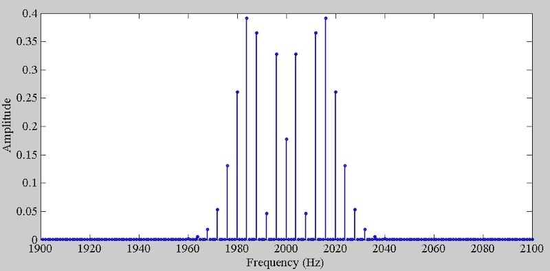
Figure 2. The spectrum of the tone-modulated FM wave when Δf = 20 Hz, f_m = 4 Hz, and β = 5.

 

Visual inspection of this output spectrum suggests that the signal's bandwidth is consistent with Carson's rule. Applying Carson's rule, the bandwidth of the signal is estimated as:

$$BW~=~2(\Delta f~+~f_m)~=~2(20~+~4)~=~48 \ \text{Hz}$$

Equation 2.

 

In this section, we'll keep f_m unchanged and vary the peak frequency deviation (Δf). We'll start by doubling the frequency deviation to Δf = 40 Hz. Applying Equation 1, we now have β = 10. Figure 3 shows the resulting output spectrum.

 

Figure 3. The spectrum of the tone-modulated FM wave when Δf = 40 Hz, f_m = 4 Hz, and β = 10.

 

Once again, we use Carson's rule to calculate the bandwidth:

$$BW~=~2(\Delta f~+~f_m)~=~2(40~+~4)~=~88 \ \text{Hz}$$

Equation 3.

 

This is much larger than our previous value. Comparing Figures 2 and 3, we see that the spacing between the output frequency components remains unchanged. This is because the tone separation is dictated by the modulating frequency, which is constant. However, doubling Δf doubles the modulation index. This increases the number of significant sidebands and, consequently, the bandwidth.

Finally, let's increase Δf to 80 Hz. With f_m = 4 Hz, we obtain β = 20 and a bandwidth of:

$$BW~=~2(\Delta f~+~f_m)~=~2(80~+~4)~=~168 \ \text{Hz}$$

Equation 4.

 

The output spectrum for this case is shown in Figure 4.

 

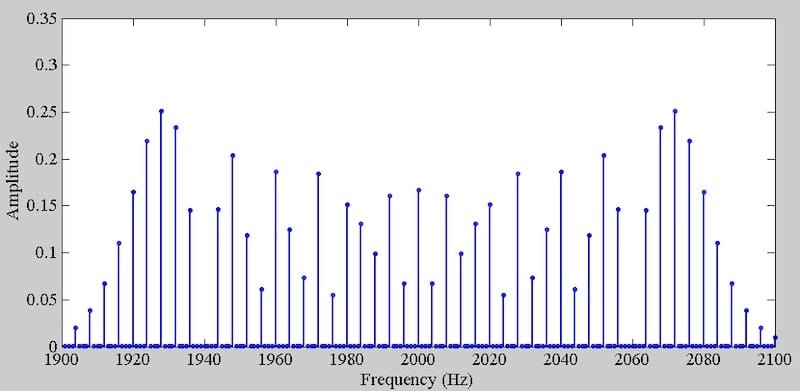
Figure 4. The spectrum of the tone-modulated FM wave when Δf = 80 Hz, f_m = 4 Hz, and β = 20.

 

With a fixed modulating frequency, the spacing between the output frequency components once again remains unchanged. As expected, increasing the frequency deviation increases the bandwidth. If f_m is small compared to Δf, we have:

$$BW~=~2(\Delta f~+~f_m)~\approx~2 \Delta f$$

Equation 5.

 

meaning that the bandwidth increases almost in direct proportion with Δf.

 

How Does the FM Wave's Bandwidth Change With Modulating Frequency?

Next, let's see what happens if we keep the frequency deviation (Δf) constant but vary the modulating frequency (f_m). The output spectrum for Δf = 20 Hz, f_m = 4 Hz, and β = 5 is shown in Figure 5.

 

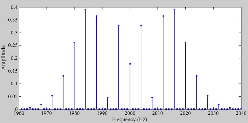
Figure 5. The spectrum of the tone-modulated FM wave for Δf = 20 Hz, f_m = 4 Hz, and β = 5.

 

Note that these are the same values we used for Figure 2. The spectrum appears slightly different because a different range is shown on the x-axis.

If we reduce the modulating frequency to f_m = 2 Hz, we obtain the spectrum in Figure 6.

 

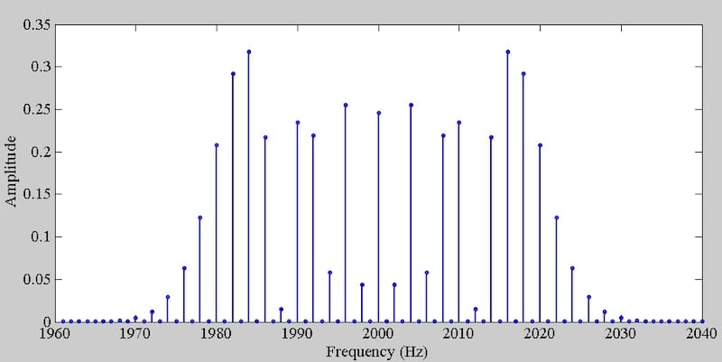
Figure 6. The FM wave spectrum for Δf = 20 Hz, f_m = 2 Hz, and β = 10.

 

As we noted previously, reducing f_m by half doubles the modulation index to β = 10. The number of significant sidebands therefore increases. However, since f_m dictates the spacing between the frequency components, the sidebands move closer to each other. As a result of this dual effect, we expect the FM bandwidth to change slightly with the modulating frequency.

Let's use Carson's rule to verify this. Recall that for Δf = 20 Hz and f_m = 4 Hz, we have:

$$BW~=~2(\Delta f~+~f_m)~=~2(20~+~4)~=~48 \ \text{Hz}$$

Equation 6.

 

With f_m = 2 Hz, we obtain:

$$BW~=~2(\Delta f~+~f_m)~=~2(20~+~2)~=~44 \ \text{Hz}$$

Equation 7.

 

Notice how Δf and f_m interact with the bandwidth in different ways: Δf greatly influences it, but f_m has little effect. In our first set of simulations, for instance, a peak frequency deviation of 20 Hz corresponded to a bandwidth of 48 Hz. When we doubled the frequency deviation to Δf = 40 Hz, the bandwidth almost doubled as well—we went from BW = 48 Hz to BW = 88 Hz. By contrast, halving f_m reduces the bandwidth only slightly (from 48 Hz to 44 Hz).

For our last simulation, we'll reduce the modulating frequency to f_m = 1 Hz. This produces the spectrum in Figure 7.

 

Figure 7. The spectrum of the FM wave for Δf = 20 Hz, f_m = 1 Hz, and β = 20.

 

We now have a bandwidth of:

$$BW~=~2(\Delta f~+~f_m)~=~2(20~+~1)~=~42 \ \text{Hz}$$

Equation 8.

 

which is only slightly less than the previous values. If we compare the bandwidths we calculated for the last three figures, we find out that reducing f_m leads to frequency components crowding into the fixed frequency interval:

$$(f_c~-~ \Delta f)~<~f~<~(f_c~+~ \Delta f)$$

Equation 9.

 

FM Bandwidth at Large β Values

Before we move on, let's examine the special case of the FM bandwidth when β approaches infinity. We determine the FM bandwidth using the same formula as before:

$$BW ~=~ 2(\Delta f ~+~ f_m)~=~2(\beta ~+~ 1)f_m ~\approx~ 2 \beta f_m ~=~ 2 \Delta f$$

Equation 10.

 

The bandwidth of the FM wave approaches 2Δf for large values of β. You can verify this by inspecting Figures 4 and 7, both of which correspond to a modulation index of β = 20.

 

Modulation Index: AM vs. FM

As a final point, I'd like to contrast the modulation index parameters of the AM and FM schemes. If we compare the tone-modulated FM signal given by:

$$s(t)~=~ A_c \cos \Big [ 2 \pi f_c t ~+~ \beta \sin(2 \pi f_m t) \Big ]$$

Equation 11.

 

with the conventional AM signal equation reproduced below:

$$s(t) ~=~ A_c \Big ( 1~+~ \mu m(t) \Big ) \cos(\omega_c t)$$

Equation 12.

 

we observe that the parameters β and μ play analogous roles in their respective modulation schemes. In both cases, they control the amount of modulation. However, they also show a notable difference: while the bandwidth of FM depends on β, the bandwidth of AM is independent of μ.

Furthermore, recall that β is directly proportional to the amplitude of the modulating signal (A_m) and inversely proportional to the modulating signal's frequency (f_m). The FM wave's bandwidth therefore depends on both A_m and f_m. This is not the case in the AM scheme.

For AM, when the message signal's maximum value doesn't exceed unity, we often enforce the constraint μ ≤ 1 to streamline the receiver. This enables us to use a simple envelope detector for demodulation. For optimal results, it's beneficial to select μ as close to unity as possible to maximize the recovered message signal's magnitude.

A larger β also results in a stronger recovered message signal in FM. While μ ≤ 1 is chosen in conventional AM, the FM scheme doesn't impose this constraint on the maximum value of β. Instead, FM imposes a constraint on β for a different reason: the occupied bandwidth of the modulated wave. From Equation 10, we know that the bandwidth of the FM wave for large β is approximately BW = 2Δf = 2βf_m. Therefore, for a given modulation frequency, the maximum value of β is determined by the permissible frequency bandwidth.

 

Wrapping Up

In this article, we examined how changes in Δf and f_m affect the bandwidth of tone-modulated FM signals. Through a series of simulations, we saw that varying Δf greatly influenced the bandwidth. By contrast, changing f_m had relatively little effect. We also learned that for large values of β, the bandwidth of the FM wave approaches 2Δf.

Finally, we compared the modulation index in AM and FM schemes. In conventional AM, we typically use a modulation index less than or equal to one (μ ≤ 1) in order to simplify the receiver. In FM, however, the maximum value of the modulation index is determined by the permissible FM bandwidth.

 

This article is Part 9 of a ten-part series on angle-modulated signals. All articles in this series are listed below in order of publication:

1. Introduction to Phase Modulation for RF Systems
2. Using Instantaneous Frequency to Represent PM and FM Signals
3. Understanding the Differences Between Phase and Frequency Modulation
4. Introduction to Narrowband Angle Modulation
5. Practical Insights Into Narrowband FM With a Single-Frequency Input
6. Introduction to Wideband FM Signals
7. Exploring Bessel Functions: Understanding the Spectrum of Tone-Modulated FM
8. Three Methods for Estimating the Transmission Bandwidth of FM Signals
9. Exploring the Relationship Between FM Wave Bandwidth and the Modulation Index
10. Estimating FM Wave Bandwidth: Solved Examples

 

Featured image used courtesy of Adobe Stock; all other images used courtesy of Steve Arar