Facebook
 Google
 GitHub
 Linkedin
The Relationship Between Rise Time and Bandwidth in Digital Signals
In this article, we’ll look at the relationship between the rise/fall time of a digital signal and its bandwidth.
When working with digital signals, what is the relationship between its bandwidth and its rise time/fall time? Check out this article to learn more.
In this article, we’ll look at the relationship between the rise/fall time of a digital signal and its bandwidth. Creating a connection between these two parameters, one from the time domain and the other from the frequency domain, allows us to more easily analyze a circuit. We’ll see that insight into both domains allows us to calculate the increase in the rise time of a signal as it goes through a system with a limited bandwidth.
Time and Frequency Domains
There are two different representations that are commonly used to analyze the operation of a circuit: the time domain and frequency domain representations. The time domain analysis is based on examining the changes a voltage or current experiences over time.
On the other hand, the frequency domain analysis represents the signals as a sum of several sinusoids with different frequencies and examines the circuit behavior in response to each of these frequency components.
Answering a particular question may become easier if we choose the suitable representation to analyze a circuit. For example, using the time-domain representation allows us to more easily understand the wave reflection phenomenon that occurs when driving a relatively long wire with a fast logic gate.
However, for example, the EMC performance of a PC board can be better analyzed if we use the frequency domain representation. Since answering a given question can be easier in one domain or another, we sometimes need to be able to translate time-domain parameters to frequency-domain parameters and vice versa.
In this article, we’ll look at the relationship between a digital signal’s rise/fall time and its bandwidth, which is a frequency-domain parameter. But before that, let’s have a look at some important concepts.
Rise Time: An Important Time Domain Parameter
The rise time of a digital signal is a very important time-domain parameter. For example, rise time can directly affect the ground bounce of a PCB. This is illustrated in Figure 1 below.
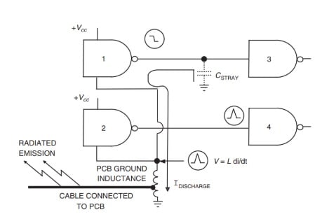
Figure 1. Image courtesy of Electromagnetic Compatibility Engineering.
In this figure, the inductance of the ground path is modeled by a lumped inductor. When the output of gate 1 goes from logic high to logic low, the electric charge stored in \[C_{STRAY}\] discharges through the ground path. This leads to a ground bounce given by \[V = \frac {\Delta I}{\Delta t}\] where \[\Delta I \] is the discharge current that flows through the ground inductance and \[\Delta t \] is the discharge time interval which is related to the rise/fall time of the gate output.
The ground bounce can lead to a noise voltage at the output of gate 2 and, if large enough, even cause an unwanted transition at the output of gate 4. This is only one example illustrating the importance of rise time in a high-speed digital design. We discussed in a previous article that a sufficiently small rise time can lead to the wave reflection phenomenon when driving a relatively long wire with a fast logic gate.
Bandwidth of a Digital Signal
Bandwidth is a common frequency domain parameter used to describe the behavior of a circuit. For example, we usually consider a 3-dB bandwidth to describe the frequency response of a filter or communication channel. As shown in Figure 2, the 3dB bandwidth of a low-pass filter is part of the frequency response that lies within 3 dB of the transfer function magnitude at DC (in this figure, the magnitude at DC is 0 dB and it drops to -3 dB at the far end of the transfer function bandwidth).
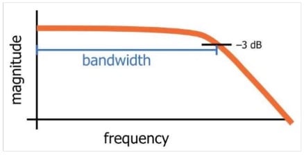
Figure 2. Image created by Robert Keim via AAC
While the above definition of bandwidth describes the behavior of a circuit, there is another definition of bandwidth that describes the frequency content of a digital signal. This definition specifies the highest significant frequency component in the spectral content of a digital signal.
We’ll explain the word “significant” used in this definition in a minute, but before that, what is the bandwidth of an ideal square wave? The spectral content of a 50% duty cycle ideal square wave (with zero rise/fall time) includes all of the odd harmonics of its fundamental frequency. For this ideal square wave, the bandwidth is infinite.
However, we cannot have this ideal signal in the real world because the device that produces this signal or the interconnect that is used to transmit it will inevitably exhibit a finite bandwidth. As a result, all of its harmonics above the 3-dB frequency of our device/interconnect will be attenuated. Due to these suppressed high-frequency harmonics, we will no longer have a zero rise time square wave. Instead, we’ll have a trapezoidal-like waveform that needs some time to transition from low to high or vice versa. Figure 3 below compares a trapezoidal signal with an ideal square wave.
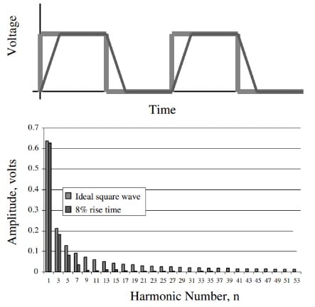
Figure 3. Image courtesy of Signal and Power Integrity-Simplified.
The above figure also shows the frequency content of the two signals. As you can see, the high-frequency harmonics in the spectrum of the trapezoidal waveform are significantly attenuated (compared to that of the ideal square wave). Since the trapezoidal waveform doesn’t have the high-frequency components, it cannot have the fast changes that are required to exhibit sharp transitions.
As discussed above, an ideal square wave has infinite bandwidth, but what is the bandwidth of the above trapezoidal waveform? The book Signal and Power Integrity-Simplified by Eric Bogatin, a well-respected PCB designer, suggests that if the magnitude of a frequency component of a trapezoidal waveform (with arbitrary rise/fall time) is attenuated by a factor greater than 0.7 compared to the same harmonic of the ideal square wave, then that frequency component is sufficiently attenuated and is not a significant frequency component in the signal spectrum. Considering only the significant frequency components, we can find the bandwidth of a given trapezoidal waveform.
For example, by visual inspection of Figure 3, we observe that the 7th harmonic is attenuated by a factor greater than 0.7 (compared to the same harmonic of the ideal square wave). Hence, this harmonic is not significant. However, the 5th harmonic seems to be significant by the above definition. Therefore, the bandwidth of this trapezoidal waveform extends from DC to the 5th harmonic. If the waveform period is 10 ns, the fundamental harmonic will be 100 MHz and the bandwidth will be 500 MHz.
Rise Time and Bandwidth
We saw that in practice, we cannot have zero rise time. The non-zero rise/fall time of a trapezoidal waveform corresponds to a limited bandwidth in the frequency domain. There is an approximation that relates the rise time of a signal to its bandwidth as:
\[BW = \frac {0.35}{T_r}\]
In this equation, \[T_r\] is the 10-90% rise time of the signal. The 10-90% rise time is the time interval it takes the signal to go from 10% of its final value to 90% of its final value. For example, if a signal has a rise time of 0.5 ns, its bandwidth will be 700 MHz.
How Does an Interconnect Change a Signal Rise Time?
In the final section of this article, let’s have a brief look at an interesting problem.
What happens if we pass a signal with a given rise time \[T_{r, in}\] through a circuit that has bandwidth BW? How does the limited bandwidth of the circuit affect the signal rise time?
For example, assume that we pass the signal through a 4-inch-long transmission line that has a bandwidth of BW. If BW is low enough, it can suppress some of the frequency components of the input signal and make them insignificant (we explained above what significant means in this context).
Since some of the high-frequency components are suppressed, the signal rise time can increase as it reaches the far end of the interconnect. Therefore, a low-bandwidth circuit/interconnect can increase the rise time of a signal.
The following equation allows us to quantify this effect:
\[T_{r,out} = \sqrt{T^2 _{r,in} + T^2 _{r,system}}\]
Here, \[T_{r, out}\] is the rise time at the interconnect output and \[T_{r, system}\] is the rise time associated with the interconnect. The interconnect rise time can be obtained from its bandwidth using the equation discussed in the previous section. For example, if an interconnect has a bandwidth of 6 GHz, we can associate a rise time of 58.3 ps (picoseconds) with this interconnect. Now, if we send a signal with \[T_{r, in} = 50 ps \] into this interconnect, the rise time of the signal would increase to 76.8 ps at the far end of the interconnect.
You can find the mathematical derivation of the above equation in Section 8.5.3 of the book The Design of CMOS Radio-Frequency Integrated Circuits. Unfortunately, the derivation of this equation is not so straightforward. Note that we can easily extend this equation to calculate the rise time at the output of N cascaded systems.
Conclusion
In this article, we discussed how insight into both time and frequency domains allows us to more easily understand the behavior of a circuit. We looked at the relationship between the rise time and bandwidth of a signal. We saw that the rise time of a signal is inversely proportional to its bandwidth and that the product of these two parameters is always approximately 0.35. We also saw that as a signal goes through a system with limited bandwidth, its rise time increases.
To see a complete list of my articles, please visit this page.
Related Content