What Is a Low Pass Filter? A Tutorial on the Basics of Passive RC Filters

What is filtering? Learn what resistor-capacitor (RC) low-pass filters are and where you can use them.

This article introduces the concept of filtering and explains in detail the purpose and characteristics of resistor-capacitor (RC) low-pass filters.

Time Domain and Frequency Domain

When you look at an electrical signal on an oscilloscope, you see a line that represents changes in voltage with respect to time. At any specific moment in time, the signal has only one voltage value. What you see on the oscilloscope is the time-domain representation of the signal.

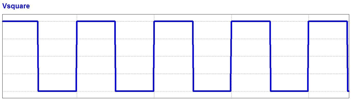
A typical oscilloscope trace is straightforward and intuitive, but it is also somewhat restrictive, because it does not directly reveal the frequency content of a signal. In contrast to the time-domain representation, in which one moment in time corresponds to only one voltage value, a frequency-domain representation (also called a spectrum) conveys information about a signal by identifying the various frequency components that are simultaneously present.

 

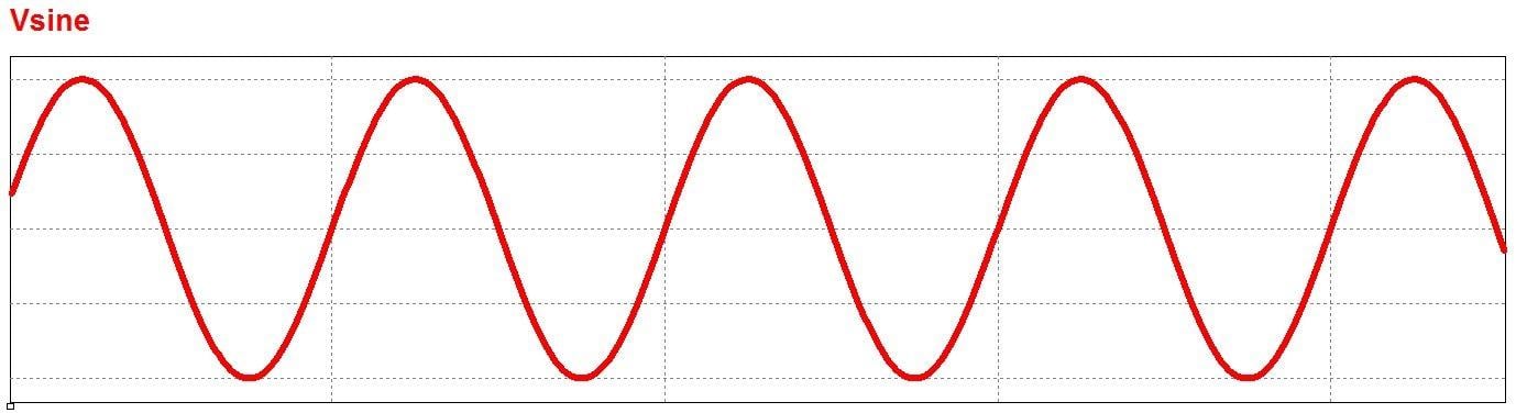
Time-domain representations of a sinusoid (top) and a square wave (bottom).

 

Frequency-domain representations of a sinusoid (top) and a square wave (bottom).

What Is a Filter?

A filter is a circuit that removes, or “filters out,” a specified range of frequency components. In other words, it separates the signal’s spectrum into frequency components that will be passed and frequency components that will be blocked.

If you don’t have much experience with frequency-domain analysis, you might still be uncertain about what these frequency components are and how they coexist in a signal that cannot have multiple voltage values at the same time. Let’s look at a brief example that will help to clarify this concept.

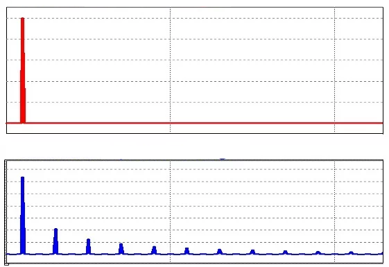
Let’s imagine that we have an audio signal that consists of a perfect 5 kHz sine wave. We know what a sine wave looks like in the time domain, and in the frequency domain we will see nothing but a frequency “spike” at 5 kHz. Now let’s suppose that we activate a 500 kHz oscillator that introduces high-frequency noise into the audio signal.

The signal as seen on an oscilloscope will still be only one sequence of voltages, with one value per moment of time, but the signal will look different because its time-domain variations must now reflect both the 5 kHz sine wave and the high-frequency noise fluctuations.

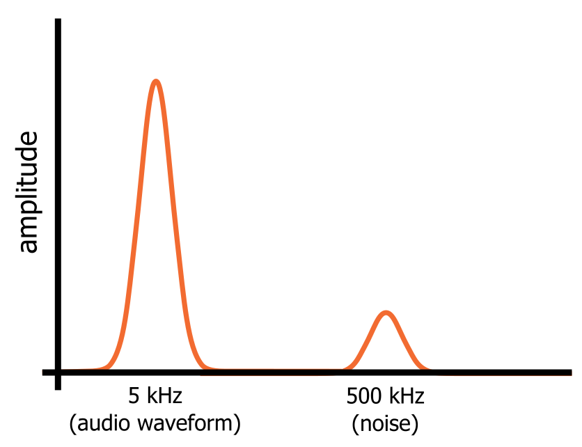
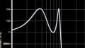
In the frequency domain, though, the sine wave and the noise are separate frequency components that are present simultaneously in this one signal. The sine wave and the noise occupy different portions of the signal’s frequency-domain representation (as shown in the diagram below), and this means that we can filter out the noise by directing the signal through a circuit that passes low frequencies and blocks high frequencies.

 

Types of Filters

Filters can be placed into broad categories that correspond to the general characteristics of the filter’s frequency response. If a filter passes low frequencies and blocks high frequencies, it is called a low-pass filter. If it blocks low frequencies and passes high frequencies, it is a high-pass filter. There are also band-pass filters, which pass only a relatively narrow range of frequencies, and band-stop filters, which block only a relatively narrow range of frequencies.

 

 

Filters can also be classified according to the types of components that are used to implement the circuit. Passive filters use resistors, capacitors, and inductors; these components have no ability to provide amplification, and consequently a passive filter can only maintain or reduce the amplitude of an input signal. An active filter, on the other hand, can both filter a signal and apply gain, because it includes an active component such as a transistor or an operational amplifier.

 

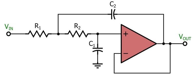
This active low-pass filter is based on the popular Sallen–Key topology.

 

This article explores the analysis and design of passive low-pass filters. These circuits play an important role in a wide variety of systems and applications.

The RC Low-Pass Filter

To create a passive low-pass filter, we need to combine a resistive element with a reactive element. In other words, we need a circuit that consists of a resistor and either a capacitor or an inductor. In theory, the resistor-inductor (RL) low-pass topology is equivalent, in terms of filtering ability, to the resistor-capacitor (RC) low-pass topology. In practice, though, the resistor-capacitor version is much more common, and consequently the rest of this article will focus on the RC low-pass filter.

 

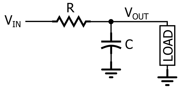
The RC low-pass filter.

 

As you can see in the diagram, an RC low-pass response is created by placing a resistor in series with the signal path and a capacitor in parallel with the load. In the diagram, the load is a single component, but in a real circuit it might be something much more complicated, such as an analog-to-digital converter, an amplifier, or the input stage of the oscilloscope that you are using to measure the response of the filter.

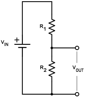
We can intuitively analyze the filtering action of the RC low-pass topology if we recognize that the resistor and the capacitor form a frequency-dependent voltage divider.

 

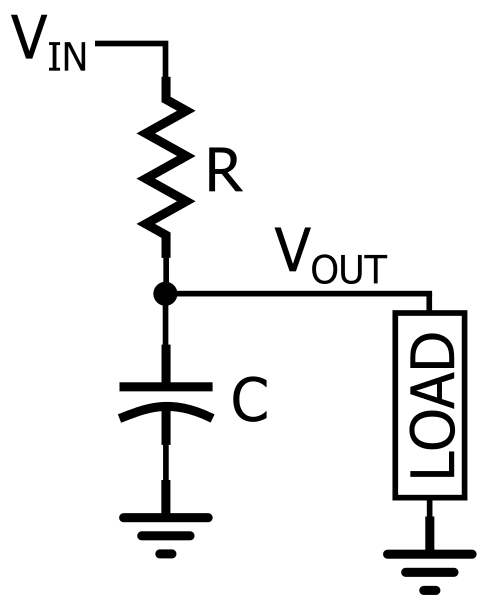
The RC low-pass filter redrawn so that it looks like a voltage divider.

 

When the frequency of the input signal is low, the impedance of the capacitor is high relative to the impedance of the resistor; thus, most of the input voltage is dropped across the capacitor (and across the load, which is in parallel with the capacitor). When the input frequency is high, the impedance of the capacitor is low relative to the impedance of the resistor, which means that more voltage is dropped across the resistor and less is transferred to the load. Thus, low frequencies are passed and high frequencies are blocked.

This qualitative explanation of RC low-pass functionality is an important first step, but it isn’t very helpful when we need to actually design a circuit, because the terms “high frequency” and “low frequency” are extremely vague. Engineers need to create circuits that pass and block specific frequencies. For example, in the audio system described above, we want to preserve a 5 kHz signal and suppress a 500 kHz signal. This means that we need a filter that transitions from passing to blocking somewhere between 5 kHz and 500 kHz.

The Cutoff Frequency

The range of frequencies for which a filter does not cause significant attenuation is called the passband, and the range of frequencies for which the filter does cause significant attenuation is called the stopband. Analog filters, such as the RC low-pass filter, always transition gradually from passband to stopband. This means that it is impossible to identify one frequency at which the filter stops passing signals and starts blocking signals. However, engineers need a way to conveniently and concisely summarize the frequency response of a filter, and this is where the concept of cutoff frequency comes into play.

When you look at a plot of an RC filter’s frequency response, you will notice that the term “cutoff frequency” is not very accurate. The image of a signal’s spectrum being “cut” into two halves, one of which is retained and one of which is discarded, does not apply, because attenuation increases gradually as frequencies move from below the cutoff to above the cutoff.

The cutoff frequency of an RC low-pass filter is actually the frequency at which the amplitude of the input signal is reduced by 3 dB (this value was chosen because a 3 dB reduction in amplitude corresponds to a 50% reduction in power). Thus, the cutoff frequency is also called the –3 dB frequency, and in fact this name is more accurate and more informative. The term bandwidth refers to the width of a filter’s passband, and in the case of a low-pass filter, the bandwidth is equal to the –3 dB frequency (as shown in the diagram below).

 

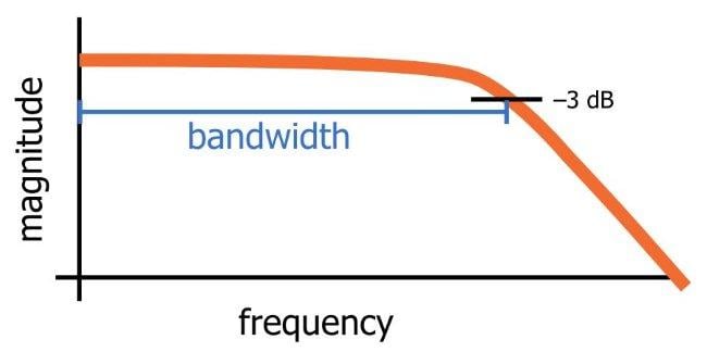
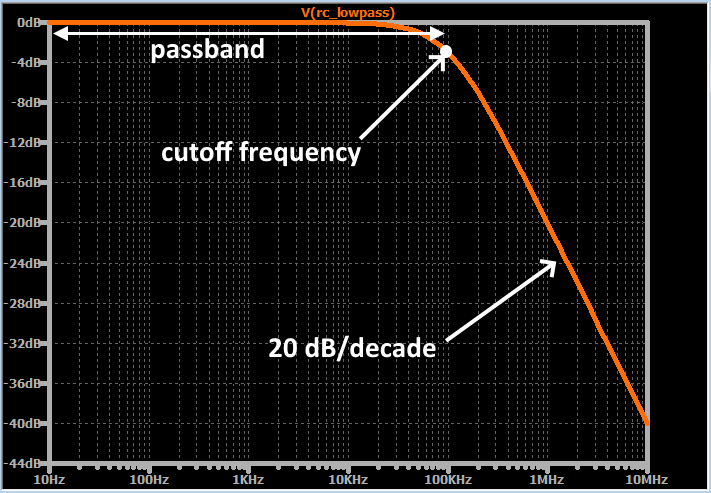
This diagram conveys the generic characteristics of the frequency response of an RC low-pass filter. The bandwidth is equal to the –3 dB frequency.

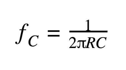
As explained above, the low-pass behavior of an RC filter is caused by the interaction between the frequency-independent impedance of the resistor and the frequency-dependent impedance of the capacitor. To determine the details of a filter’s frequency response, we need to mathematically analyze the relationship between resistance (R) and capacitance (C), and we can also manipulate these values in order to design a filter that meets precise specifications. The cutoff frequency (f_C) of an RC low-pass filter is calculated as follows:

 

 

Let’s look at a simple design example. Capacitor values are more restrictive than resistor values, so we’ll start with a common value of capacitance (such as 10 nF), and then we’ll use the equation to determine the required resistance value. The goal is to design a filter that will preserve a 5 kHz audio waveform and reject a 500 kHz noise waveform. We’ll try a cutoff frequency of 100 kHz, and later in the article we’ll more carefully analyze the effect of this filter on the two frequency components.

 

 

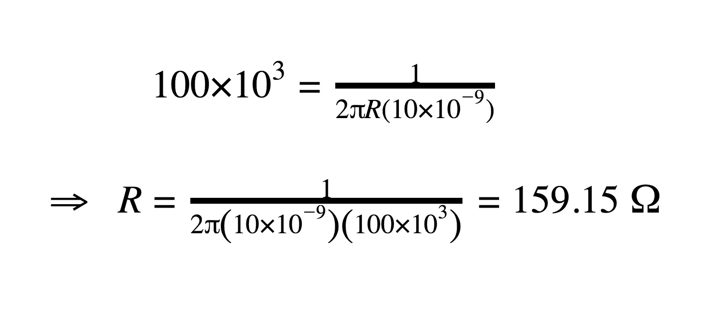
Thus, a 160 Ω resistor combined with a 10 nF capacitor will give us a filter that closely approximates the desired frequency response.

Calculating Filter Response

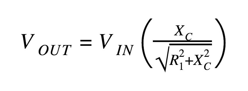
We can calculate the theoretical behavior of a low-pass filter by using a frequency-dependent version of a typical voltage-divider calculation. The output of a resistive voltage divider is expressed as follows:

 

 

 

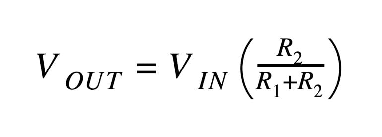
The RC filter uses an equivalent structure, but instead of R₂ we have a capacitor. First, we replace R₂ (in the numerator) with the reactance of the capacitor (X_C). Next, we need to calculate the magnitude of the total impedance and place that in the denominator. Thus, we have

 

 

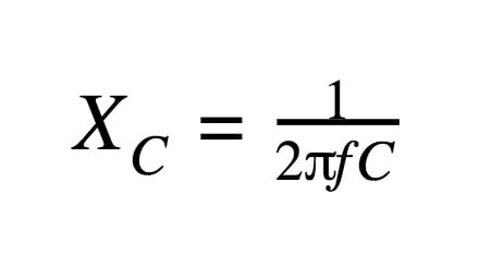
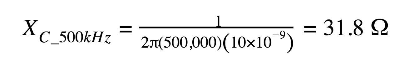
The reactance of a capacitor indicates the amount of opposition to current flow, but unlike resistance, the amount of opposition depends on the frequency of the signal passing through the capacitor. Thus, we have to calculate reactance at a specific frequency, and the equation that we use for this is the following:

 

 

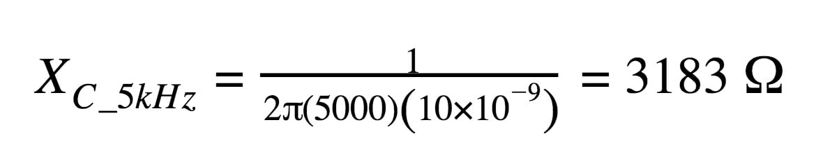
In the design example above, R ≈ 160 Ω and C = 10 nF. We’ll assume that the amplitude of V_IN is 1 V, so that we can simply remove V_IN from the calculation. First let’s calculate the amplitude of V_OUT at the sine-wave frequency:

 

 

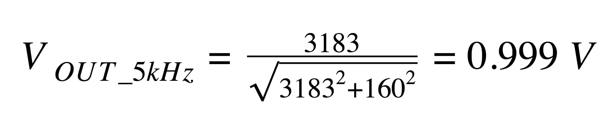
The amplitude of the sine wave is essentially unchanged. That’s good, since our intention was to preserve the sine wave while suppressing the noise. This result is not surprising, since we chose a cutoff frequency (100 kHz) that is much higher than the sine-wave frequency (5 kHz).

Now let’s see how successfully the filter will attenuate the noise component.

 

 

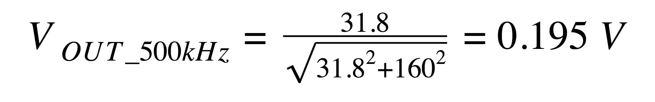
The noise amplitude is only about 20% of its original value.

Visualizing Filter Response

The most convenient means of evaluating a filter’s effect on a signal is to examine a plot of the filter’s frequency response. These graphs, often called Bode plots, have magnitude (in decibels) on the vertical axis and frequency on the horizontal axis; the horizontal axis typically has a logarithmic scale, such that the physical distance between 1 Hz and 10 Hz is the same as the physical distance between 10 Hz and 100 Hz, between 100 Hz and 1 kHz, and so forth. This configuration allows us to quickly and accurately assess the behavior of a filter over a very large range of frequencies.

 

An example of a frequency-response plot.

 

Each point on the curve indicates the magnitude that the output signal will have if the input signal has a magnitude of 1 V and a frequency equal to the corresponding value on the horizontal axis. For example, when the input frequency is 1 MHz, the output amplitude (assuming an input amplitude of 1 V) will be 0.1 V (because –20 dB corresponds to a factor-of-ten reduction).

The general shape of this frequency-response curve will become very familiar as you spend more time with filter circuits. The curve is almost perfectly flat in the passband, and then it begins to drop more rapidly as the input frequency approaches the cutoff frequency. Eventually the rate of change in attenuation, called the roll-off, stabilizes at 20 dB/decade—that is, the magnitude of the output signal is reduced by 20 dB for every factor-of-ten increase in input frequency.

 

Assessing Low-Pass Filter Performance

If we carefully plot the frequency response of the filter that we designed earlier in the article, we will see that the magnitude response at 5 kHz is essentially 0 dB (i.e., almost zero attenuation) and the magnitude response at 500 kHz is approximately –14 dB (which corresponds to a gain of 0.2). These values are consistent with the results of the calculations that we performed in the previous section.

Because RC filters always have a gradual transition from passband to stopband, and because the attenuation never reaches infinity, we cannot design a “perfect” filter—that is, a filter that has no effect on the sine wave and completely eliminates the noise. Instead, we always have a trade-off. If we move the cutoff frequency closer to 5 kHz, we will have more noise attenuation but also more attenuation of the sine wave that we want to send to a speaker. If we move the cutoff frequency closer to 500 kHz, we’ll have less attenuation at the sine-wave frequency, but also less attenuation at the noise frequency.

Low-Pass Filter Phase Shift

So far we have discussed the way in which a filter modifies the amplitude of the various frequency components in a signal. However, reactive circuit elements always introduce phase shift in addition to amplitude effects.

The concept of phase refers to the value of a periodic signal at a specific moment within a cycle. Thus, when we say that a circuit causes phase shift, we mean that it creates a misalignment between the input signal and the output signal: the input and output signals no longer begin and end their cycles at the same moment in time. The phase shift value, such as 45° or 90°, indicates how much misalignment has been created.

Each reactive element in a circuit introduces 90° of phase shift, but this phase shift does not happen all at once. The phase of the output signal, just like the magnitude of the output signal, changes gradually as the input frequency increases. In an RC low-pass filter, we have one reactive element (the capacitor), and consequently the circuit will eventually introduce 90° of phase shift.

As with magnitude response, phase response is most easily evaluated by examining a plot in which the horizontal axis indicates logarithmic frequency. The description below conveys the general pattern, and then you can fill in the details by examining the plot.

• Phase shift is initially 0°.
• It gradually increases until it reaches 45° at the cutoff frequency; during this portion of the response, the rate of change is increasing.
• After the cutoff frequency, the phase shift continues to increase, but the rate of change is decreasing.
• The rate of change becomes very small as the phase shift asymptotically approaches 90°.

 

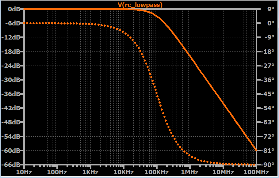
The solid line is the magnitude response, and the dotted line is the phase response. The cutoff frequency is 100 kHz. Note that the phase shift is 45° at the cutoff frequency.

Second-Order Low-Pass Filters

Thus far we have assumed that an RC low-pass filter consists of one resistor and one capacitor. This configuration is a first-order filter.

The “order” of a passive filter is determined by the number of reactive elements—i.e., capacitors or inductors—that are present in the circuit. A higher-order filter has more reactive elements, and this leads to more phase shift and steeper roll-off. This second characteristic is the primary motivation for increasing the order of a filter.

By adding one reactive element to a filter—e.g., by going from first-order to second-order or second-order to third-order—we increase the maximum roll-off by 20 dB/decade. Steeper roll-off translates into a more rapid transition from low attenuation to high attenuation, and this can result in improved performance when the signal does not have a wide frequency band that separates the desired frequency components from the noise components.

Second-order filters are commonly built around a resonant circuit consisting of an inductor and a capacitor (this topology is called “RLC” for resistor-inductor-capacitor). However, it is also possible to create second-order RC filters. As shown in the diagram below, all we need to do is cascade two first-order RC filters.

 

 

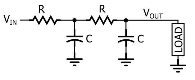
Though this topology certainly does create a second-order response, it is not widely used—as we’ll see in the next section, the frequency response is often inferior to that of a second-order active filter or a second-order RLC filter.

Frequency Response of the Second-Order RC Filter

We can attempt to create a second-order RC low-pass filter by designing a first-order filter according to the desired cutoff frequency and then connecting two of these first-order stages in series. This does result in a filter that has a similar overall frequency response and a maximum roll-off of 40 dB/decade instead of 20 dB/decade.

However, if we look at the response more closely, we see that the –3 dB frequency has decreased. The second-order RC filter does not behave as expected because the two stages are not independent—we cannot simply connect these two stages together and analyze the circuit as a first-order low-pass filter followed by an identical first-order low-pass filter.

Furthermore, even if we insert a buffer between the two stages, so that the first RC stage and the second RC stage can function as independent filters, the attenuation at the original cutoff frequency will be 6 dB instead of 3 dB. This occurs precisely because the two stages are operating independently—the first filter has 3 dB of attenuation at the cutoff frequency, and the second filter adds another 3 dB of attenuation.

 

 

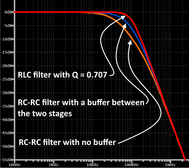
The fundamental limitation of the second-order RC low-pass filter is that the designer cannot fine-tune the transition from passband to stopband by adjusting the filter’s Q factor; this parameter indicates how damped the frequency response is. If you cascade two identical RC low-pass filters, the overall transfer function corresponds to a second-order response, but the Q factor is always 0.5. When Q = 0.5, the filter is on the border of being overdamped, and this results in a frequency response that “sags” in the transition region. Second-order active filters and second-order resonance-based filters do not have this limitation; the designer can control the Q factor and thereby fine-tune the frequency response in the transition region.

Summary

• All electrical signals contain a mixture of desired frequency components and undesired frequency components. The undesired frequency components are typically caused by noise and interference, and in some situations they will negatively affect the performance of the system.
• A filter is a circuit that reacts in different ways to different portions of a signal’s spectrum. A low-pass filter is designed to pass low-frequency components and block high-frequency components.
• The cutoff frequency of a low-pass filter indicates the frequency region in which the filter is transitioning from low attenuation to significant attenuation.
• The output voltage of an RC low-pass filter can be calculated by treating the circuit as a voltage divider consisting of a (frequency-independent) resistance and a (frequency-dependent) reactance.
• A plot of magnitude (in dB, on the vertical axis) versus logarithmic frequency (in hertz, on the horizontal axis) is a convenient and effective way to examine the theoretical behavior of a filter. You can also use a plot of phase versus logarithmic frequency to determine the amount of phase shift that will be applied to an input signal.
• A second-order filter provides steeper roll-off; this second-order response is helpful when a signal does not provide a wide band of separation between desired frequency components and undesired frequency components.
• You can create a second-order RC low-pass filter by building two identical first-order RC low-pass filters and then connecting the output of one to the input of the other. The overall –3 dB frequency will be lower than expected.