 Facebook
 Google
 GitHub
 Linkedin
Implementing a Low-Pass Filter on FPGA with Verilog
Learn how to implement a moving average filter and optimize it with CIC architecture.
In this article, we'll briefly explore different types of filters and then learn how to implement a moving average filter and optimize it with CIC architecture.
Filtering is very important in many designs. It provides us with an opportunity to extract the desired signal buried underneath a lot of noise. We can also determine the non-linearity of a system by filtering its output at certain frequencies.
Let's start by discussing some differences between types of filters.
Theory
Types of Filters
Filters can be categorized into one of five groups according to their band class. What each one is capable is hinted at in their name. For example, a low-pass filter is a filter that passes low-frequency inputs and blocks high-frequency ones and etc.
The five types are:
- Low-pass
- Band-pass
- Band-stop
- High-pass
- All-pass
Filters also come in different shapes. For example, they may have ripple on their pass-band or they may have a flat transition band, etc.
Filter Shape
Filters can typically be categorized by shape as follows:
- Bessel: the flattest group delay compared to the others
- Butterworth: are designed to have the flattest magnitude frequency response in the passband; are also called "maximally flat"
- Chebyshev: designed to have the minimum error between an ideal filter and real filter; can be categorized into two types: those with a ripple in the pass band and those with a ripple in the stopband
- Elliptic: have ripples in both the pass and stop bands, but also they have the fastest transition between pass and stop band
Choosing the shape of filter relies on the desired specifications. For example, we may need the output signal amplitude to follow the input signal amplitude in the pass band as precisely as possible. In this case, we should use a Butterworth filter even it will give us more transition band.
On the other hand, we may want output signal frequency to follow the input signal exactly with a linear phase response, so we should choose Bessel filters. In cases where we need to use as few components as possible and have the same order and transition speed as other filters, an Elliptic or Chebyshev filter would work, but we get a ripple in the pass or stop band.
Analog and Digital Filters
In another aspect, filters can be constructed in two ways: digital and analog.
In an analog circuit, passive filters are a ladder of inductors and capacitors or resistors. Active analog filters can be a structure that exploits amplifiers or resonators. Their value can be determined simply by using tables or applications already created for designing analog filters.
Digital filters can be created with two methods, IIR and FIR. IIR (infinite impluse response) filters are the types of filters in which the output depends on the inputs and previous outputs.
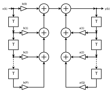
Figure 1. IIR filter. Image courtesy of Mark Wilde [CC BY-SA 3.0]
Another type of filter implementation of digital filters is FIR (finite impulse response). These do not use feedback and their output is only related to current and previous inputs. With regard to stability, FIR filters are always stable because their output is only related to inputs. On the other hand, they need a higher order to meet the same specifications as IIRs.
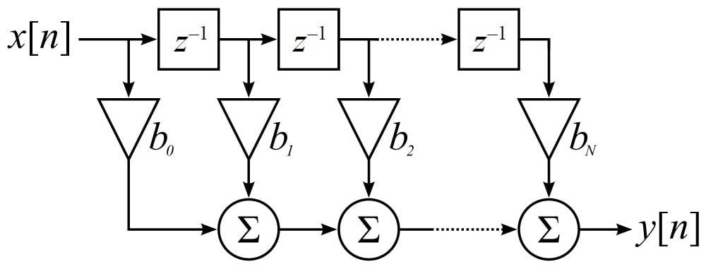
Figure 2. FIR filter Image courtesy of Jonathan Blanchard
Moving Average
Moving average is a filter that averages N points of previous inputs and makes an output with them.
$$ y[n]= \frac{1}{N}\sum_{i=0}^{N} x_{n-i} $$
As you can see, the moving average filter is a FIR filter with N coefficients of $$\frac{1}{N}$$. The frequency response of some moving average filters with different N is shown in Figure 3.
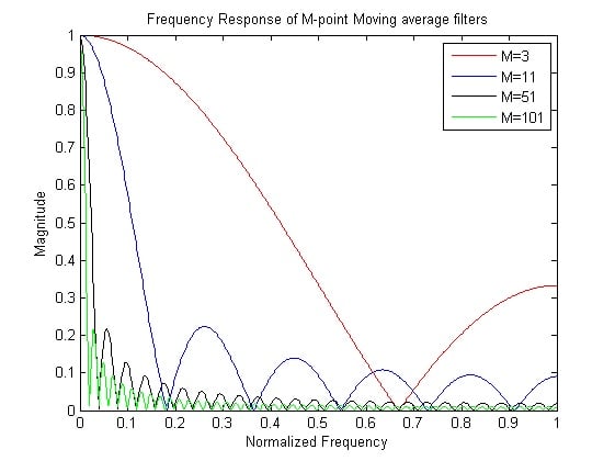
Figure 3. Frequency response of moving average
Impulse response of a moving average (MA) filter is zero in the points which are not inside 0 to N.
$$h[n] = \frac{1}{N}\sum_{k=0}^{N-1} \delta[n-k]$$
So, the frequency response of an MA filter is:
$$\begin{align}H(\omega) &= \frac{1}{N} \frac{e^{-j \omega N/2}}{e^{-j \omega/2}} \frac{j2 \sin\left(\frac{\omega N}{2}\right)}{j2 \sin\left(\frac{\omega}{2}\right)} \\&=\frac{1}{N} \frac{e^{-j \omega N/2}}{e^{-j \omega/2}} \frac{\sin\left(\frac{\omega N}{2}\right)}{\sin\left(\frac{\omega}{2}\right)}\end{align}$$
And cut-off frequency can be estimated as:
$$F_{co} = \frac {0.442947} {\sqrt{N^2-1}}$$
According to these formulas, cut-off frequency only relates to the N. As N increases, the cut-off frequency decreases but with a cost of time. We need to wait for the Nth cycle to get the correct result, so with larger N, we need more time. As a filter gets sharper, the time its output needs to reach steady state increases.
Filtering and implementation of the desired design are broad topics in FPGA design. One needs to learn a lot to design an appropriate filter and then implement it on FPGA with minimum resource usage or fastest possible speeds.
In this article, we will try to implement an N-point moving average filter. We'll assume N is a parameter which can be changed before implementation by CAD tools such as Xilinx ISE.
As we can see in Figure 2, a FIR filter can be implemented by a delay chain with the length of N, which is the FIR order, multipliers that multiply coefficients to the delay line, and some adders which add the multipliers' results. This architecture needs many multipliers and adders, which are limited in FPGAs, depending on which FPGA you're using (though even the most powerful FPGAs are limited, too).
Designing FIR filters requires some research to reduce these resources because, in every stage of the design with any FPGA, reduction is necessary. However, we won’t cover this topic—instead, we'll design our moving average filter with another trick. In a moving average filter, all coefficients are $$\frac{1}{N}$$. If we want to implement our filter like Figure 2, we should make a tap delay line and store N last inputs, then multiply them with $$\frac{1}{N}$$ and finally sum the results. However, we can store N last inputs in a FIFO and add them and then multiply them by 1/N in each cycle. With this approach, we only need one N multiplier.
Code Description
First, we have N, which is the number of input points as a parameter that can be tuned. We will add these N points to produce the output.
We also assumed our input is in a 28-bit format and we want the same format for output. When dealing with adding N points, we may face bit growth. Adding two 28-bit points results in a 28-bit output and one overflow bit. Therefore, for adding N 28-bit point, we need a (log2 (N) +28)-bit output.
Assume all N points are the same and adding them is like multiplying N to one of them. That is why we implement a “log2” function which simply calculates the logarithm of its input. By knowing the logarithm of N, we can set the output length. Note that log2 is not a synthesizable method and will only work on Xilinx ISE (i.e., Xilinx ISE calculates log2 and then will use the result for the rest of the implementation).
“log2” function is illustrated in the code below:
function integer log2(input integer v); begin log2=0; while(v>>log2) log2=log2+1; end endfunctionNow that we set our input and output length, we need to make a tap line that stores N previous and current inputs. The following code will do the trick:
genvar i;
generate
	 for (i = 0; i < N-1 ; i = i + 1) begin: gd
		 always @(posedge clock_in) begin
		 	if(reset==1'b1)
			begin
				data[i+1]<=0;
			end
			else
			begin
				data[i+1] <= data[i];
			end
		 end
    end
endgenerate
Finally, we need an adder to sum all of the data stored in the FIFO. This stage is a little tricky. If we want to have the output on every clock cycle, we need to make a combinational circuit that adds the data in the FIFO step by step. The code shown below will do this:
genvar c;
generate
	 assign summation_steps[0] = data[0] + data[1];
	 for (c = 0; c < N-2 ; c = c + 1) begin: gdz
		assign summation_steps[c+1] = summation_steps[c] + data[c+2];
    end
endgenerate
However, our target FPGA (XC3S400) doesn’t have this many resources and synthesizing this module on this FPGA is not feasible. So, I made the problem a little simpler. I assumed that we want the output to get updated every N clock cycles. With this trick, we don’t need to store all received data anymore. We can simply store the summation and add it to the current input in every cycle. The below code will do the trick:
always@(posedge clock_in)
begin
    if(reset)
    begin
        signal_out_tmp<=0;
        count<=0;
        signal_out<=0;
    end
    else
    begin
        if(down_sample_clk==N_down_sample)
        begin
            if(count             begin
                count<=count+1'b1;
                signal_out_tmp<=signal_out_tmp+signal_in;
            end
            else
            begin
                count<=0;
                signal_out<=signal_out_tmp[27+N2:N2];
                signal_out_tmp<=0;
            end
        end
    end
end
In this code, the total sum is saved as signal_out_tmp and will be added to the input every cycle. After N points, the output will become signal_out_tmp and this variable will be set to zero and start to store the sum again.
This approach uses very low resources but its output will be updated every N cycles.
Simulation
Because of its speed, we'll do a simulation using Modelsim. We need to integrate Modelsim to Xilinx ISE. In order to do this, go to Edit > Preferences > Integrated Tools. In the Model Tech Simulator section, we enter the Modelsim location and we are done, as can be seen in Figure 4.
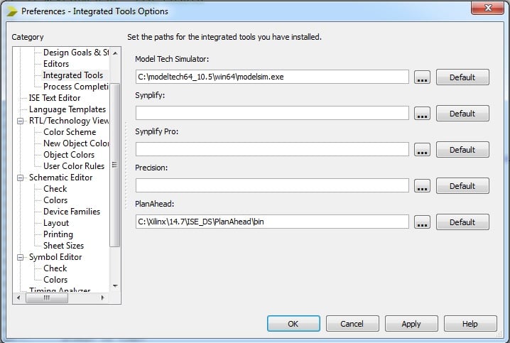
Figure 4. Setting model tech simulator
Modelsim needs to use XILINX ISE libraries in order to be able to simulate circuits. In order to do that, we need to click on FPGA model on the project and then select Compile HDL Simulation Libraries, as seen in Figure 5.
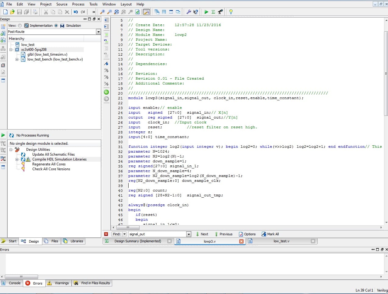
Figure 5. Compile HDL simulation libraries
The test bench is included in the project code, which you can download. In the test bench, we assumed input as a step and saved the output. Reading and writing in a test bench is very simple, as can be seen in the code below. We can open a file with the fopen function in the test bench and then write to it with the fwrite function.
f = $fopen("output.txt","w");
f2 = $fopen("time.txt","w");
$fwrite(f,"%d %d\n",signal_in,signal_out);
$fwrite(f2,"%d\n",cur_time);
Formatting in fwrite is much like a simple printf function in C language. We will also use the $time variable in the test bench. Using the $time variable gives us current time which can be written to a text file. After simulating our project, we can use the written files in MATLAB to make sure they are correct. Code written in MATLAB first reads the files and plots them.
A = importdata('D:\low_test\output.txt');
B = importdata('D:\low_test\time.txt');
M2=A(:,2);
M1=A(:,1);
T=B(:,1)*10e-9;

M1=M1/(2^24);
M2=M2/(2^24);
plot(M1);
hold on;
plot(M2);

s=size(M1);
val=0;
t=0:s(1,1)-1;
t=t*50e-9;
for i=405:s(1,1)
    if(abs(M1(i,1)-M2(i,1))<1*.1)
        val=i;
        break;
    end
end
stepp=stepinfo(M2,t);
pp=stepp.RiseTime;
fc=.35/pp
cycles=val-405
time=((cycles)*50)/1000
For testing purposes, we'll first simulate our bench with input step and then we change the input to sine. Plots are shown in Figure 6 and Figure 7.
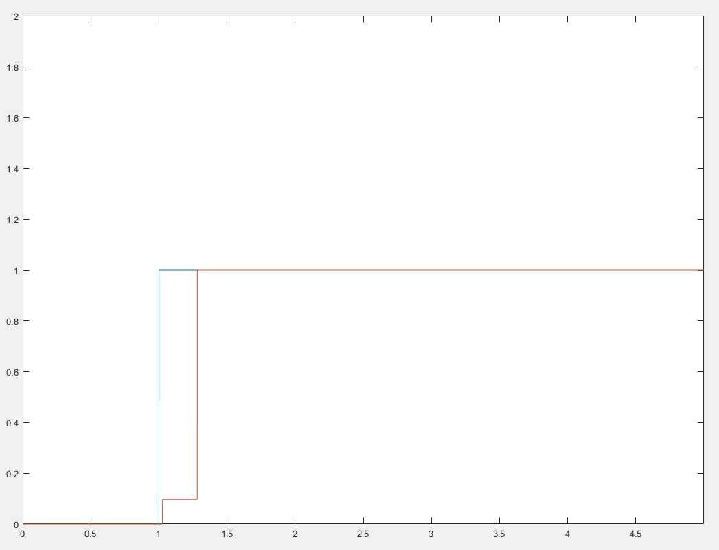
Figure 6. Step response
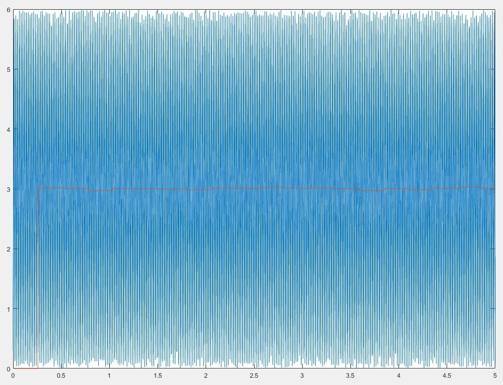
Figure 7. Sin(x)*sin(x) response
As can be seen in Figure 6, after 0.2 ms the filter output became as high as the input amplitude. Responding in every N cycles is obvious in Figure 6 because the output doesn't change smoothly. Instead, it changes after the Nth cycle.
In Figure 7, because the input is 6*sin(x)*sin(x) we know that the DC offset of this input is 3, as our low-pass filter output is 3.
CIC Filters
The cascaded integrator-comb filter is a hardware-efficient FIR digital filter.
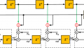
A CIC filter consists of an equal number of stages of ideal integrator filters and decimators. A CIC filter architecture can be seen in Figure 8.
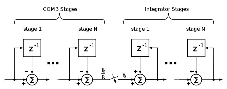
Figure 8. CIC filter image. Via Wikimedia Commons
We can optimize our moving average low-pass filter by using CIC filters and rewriting moving average equation as seen below:
$${\begin{aligned}y[n]&=\sum _{{k=0}}^{{N-1}}x[n-k]\\&=y[n-1]+x[n]-x[n-N].\end{aligned}}$$
This architecture consists of a comb section (c[n]=x[n]-x[n-N]) and an integrator (y[n]=y[n-1]+c[n]) so we can use CIC architecture here. In this architecture, we reduced adders to only three sections so that we can have the output at every cycle, which is the magic of CIC filters.
In the second code available for download, a moving average is optimized using CIC filter topology. We can implement the above equation in hardware using the following Verilog code:
wire signed [27+N2:0] signal_out_tmp_2=signal_out_tmp_3+signal_in-data[N-1];The output of the new structure with a sin(x)*sin(x) input is shown in Figure 9.
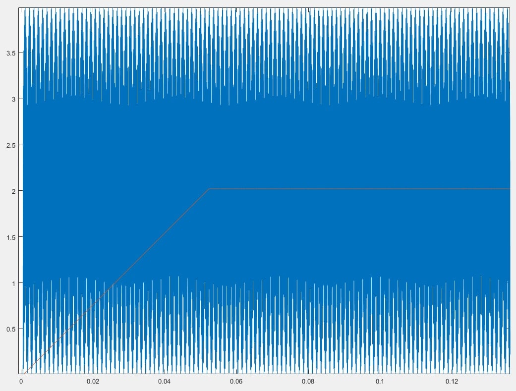
Figure 9. CIC output
Modelsim simulation of our CIC moving average filter is illustrated in the below video.
Conclusion
Both digital and analog routes work for filtering. Each has its own advantages but digital filtering allows for re-programmability and smaller implementation area. In this article, we first examined the ways that filters can be built and then we implemented a moving average filter in the simplest way. Finally, we optimized it with the CIC architecture.


Online VLSI Tutorial - Verilog RTL coding Synthesis You can also refer to the video https://youtu.be/uUZceAfnVNk for a great understanding of #verilog. This tutorial covers registers, unwanted latches & operator synthesis and helps you master these fundamental concepts.Check out the series of free tutorials by Mr. P R Sivakumar(CEO, Maven Silicon) on basic and advanced concepts of Front End VLSI. His amazing explanations and easy to understand content make these videos a great tool for you to update and upgrade your VLSI skills.
TestBench for LPF
why when i tried to run the code it didn’t have results like what you have here ??