Introduction to Narrowband Angle Modulation

As we know from earlier articles in this series, there are two forms of angle modulation: phase modulation (PM) and frequency modulation (FM). To effectively transmit and receive either type of signal, it’s essential to know the bandwidth that the modulated wave occupies. We refer to angle-modulated waves with low modulation indices as ‘narrowband.’

In this article, we’ll advance our discussion of angle modulation by exploring the spectra produced by these narrowband signals. In doing so, we’ll introduce concepts that are fundamental not just for understanding the bandwidth requirements of FM and PM waves, but also for analyzing the linearity performance of certain RF circuits.

 

Review of Angle-Modulated Signals

A constant-amplitude, angle-modulated signal is represented by the following equation:

$$s(t) ~=~ A_c \cos( 2 \pi f_c t ~+~ \phi(t) )$$

Equation 1.

 

where:

A_c is the carrier amplitude

f_c is the carrier frequency

ϕ(t) is the phase deviation.

Equation 2 illustrates the relationship between ϕ(t) and the message signal for PM schemes:

$$\phi (t) ~=~ k_p m(t)$$

Equation 2.

 

where m(t) is the message signal and k_p is the modulation index.

Equation 3 does the same for FM schemes:

$$\phi (t) ~=~ 2 \pi k_f \int_{0}^{t} m(\tau) \ d \tau$$

Equation 3.

 

Given that the message signal is the argument of the sinusoidal function, it’s clear that the modulated wave’s dependence on the message signal is nonlinear.

 

Narrowband Angle-Modulated Waves

We previously defined ‘narrowband’ as referring to a low modulation index. More precisely, the term applies to the special case of |ϕ(t)| being much smaller than 1 radian. To derive the equation for a narrowband angle-modulated wave, we first expand Equation 1 by applying a basic trigonometric identity:

$$s(t) ~=~ A_c \cos( 2 \pi f_c t) \cos(\phi(t) ) ~-~ A_c \sin( 2 \pi f_c t) \sin(\phi(t) )$$

Equation 4.

 

If |ϕ(t)| is much smaller than 1 radian, we can use the following approximations:

$$\cos(\phi(t) ) ~\approx~ 1 \quad \text{and} \quad \sin(\phi(t) ) ~\approx~ \phi(t)$$

Equation 5.

 

Invoking these approximations, Equation 4 simplifies to:

$$s(t) ~\approx~ A_c \cos( 2 \pi f_c t) ~-~ A_c \phi(t) \sin(2 \pi f_c t)$$

Equation 6.

 

This expression is similar to the equation for conventional amplitude modulation (AM), which is reproduced below:

$$s_{AM}(t) ~=~ A_c \Big ( 1~+~ \mu m(t) \Big ) \cos(\omega_c t)$$

Equation 7.

 

In both narrowband angle-modulated waves and conventional AM, the in-phase component contains a significant unmodulated carrier. For AM, the in-phase component also includes the message information. For a narrowband angle-modulated signal, the message information is contained in the quadrature component.

To determine the spectrum of the angle-modulated wave, we apply the Fourier transform to Equation 6, resulting in:

$$S(f) ~=~ \frac{A_c}{2} \big [ \delta(f~-~f_c)~+~ \delta(f~+~f_c) \big ] ~-~\frac{A_c}{2j} \big [ \Phi(f~-~f_c) ~-~ \Phi (f~+~f_c) \big ]$$

Equation 8.

 

If you struggle to derive the preceding equation, keep in mind that the sine function can be written as:

$$\sin( 2 \pi f_c t) ~=~ \frac{1}{2j} (e^{j 2 \pi f_c t} ~-~ e^{-j 2 \pi f_c t} )$$

Equation 9.

 

Furthermore, the frequency-shifting property of the Fourier transform states that if X(f) is the Fourier transform of x(t), we then have:

$$e^{j \omega_0 t} x(t) \quad \overset{\text{FT}}{\longleftrightarrow} \quad X(\omega ~-~ \omega_0)$$

Equation 10.

 

Using Equations 9 and 10, you can easily derive the output spectrum of the narrowband angle-modulated wave. However, we’ll continue to use Equation 8 in the rest of this article.

 

Example: Comparing Narrowband Angle-Modulated and AM Spectra

To get a sense of the spectra generated by narrowband FM and PM waves, let’s consider the message signal spectrum in Figure 1(a). This spectrum corresponds to a sinc function in the time domain.

 

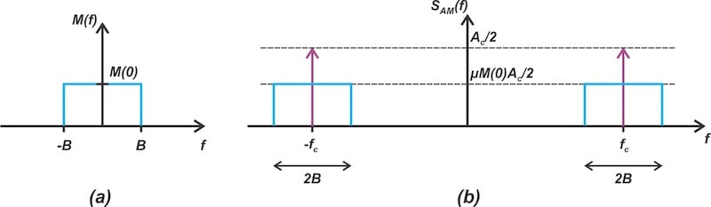
Figure 1. The spectrum of a sinc message signal (a) and of the corresponding conventional AM wave (b).

 

Applying Equation 7 to this message signal produces a conventional AM wave, the spectrum of which is illustrated in Figure 1(b). Next, let’s find the spectra generated by narrowband PM and FM schemes.

 

The Narrowband PM Spectrum

Figure 2(b) shows the spectrum of the PM wave corresponding to Figure 1(a)’s message signal. The spectrum of ϕ(t), as per Equation 2, is shown in Figure 2(a).

 

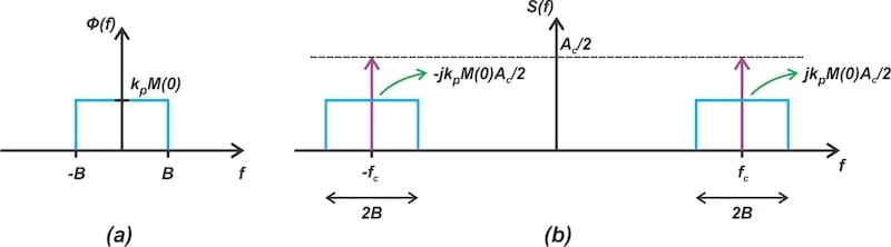
Figure 2. The spectrum of ϕ(t) for the PM scheme (a) and the spectrum of the PM wave for the sinc message signal (b).

 

Comparing Figure 2(b) with Figure 1(b), we observe that both spectra have impulse functions at ±f_c and contain replicas of the message spectrum. However, the narrowband PM spectrum is multiplied by the factor j for frequencies greater than zero and by –j for f < 0.

The factors ±j indicate a phase shift of 90 degrees with respect to the carrier frequency. The carrier has a real value because it’s contained in the in-phase component of Equation 6. By contrast, the message information has a complex value because it resides in the quadrature component.

The 3D diagram in Figure 3 provides a more accurate representation of the spectrum in Figure 2(b).

 

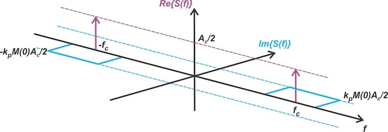
Figure 3. A 3D representation of the example PM wave’s spectrum.

 

The Narrowband FM Spectrum

To find the narrowband FM spectra, we first determine the spectrum of ϕ(t) by applying a Fourier transform to Equation 3. Using the integration property of the Fourier transform, we obtain:

$$\begin{eqnarray}\Phi (f) &~=~& 2 \pi k_f ~\times~ \mathcal{F} \Big [ \int_{-\infty}^{t} m(\tau) \ d \tau \Big ] \\&~=~& 2 \pi k_f ~\times~ \frac{1}{j 2 \pi f} ~\times~ M(f) \\&~=~& - \frac{j k_f}{f} ~\times~ M(f)\end{eqnarray}$$

Equation 11.

 

Note that the Fourier transform of the integral of a function generates an impulse function. For the sake of simplicity, this impulse function is disregarded in the above equation.

Figure 4 illustrates the derivation of Φ(f) from M(f) according to Equation 11.

 

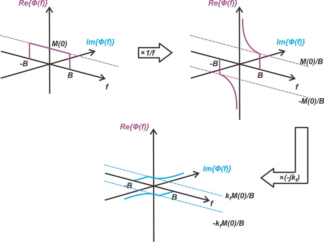
Figure 4. The spectrum of Φ(f) for the FM scheme, illustrated in 3D. [click to enlarge]

 

Due to the integration, the spectrum of Φ(f) takes the form of a truncated hyperbola in the imaginary plane. When the narrowband angle modulation equation is applied, this imaginary component is multiplied by the factor A_c/2j, converting it back into a real component. We then obtain the narrowband FM spectrum depicted in Figure 5(b).

 

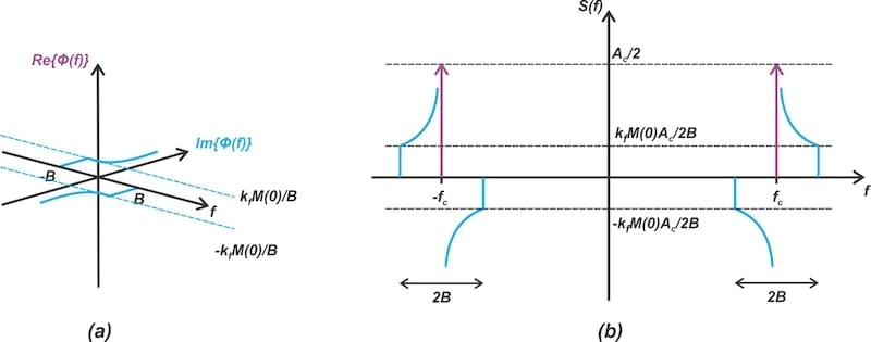
Figure 5. The spectrum of ϕ(t) for the FM scheme (a) and the spectrum of the narrowband FM wave (b).

 

Because the imaginary components of Φ(f) revert to a real component when the narrowband FM equation is applied, I used a 2D diagram to represent the final spectrum.

 

Bandwidth of Narrowband Angle-Modulated Waves

In the above example, the narrowband PM and FM schemes occupy a bandwidth of 2B, where B is the message bandwidth. Let’s see if we can use this to draw some general conclusions about the bandwidth of narrowband angle-modulated signals.

We know that narrowband angle modulation produces replicas of Φ(f) around the carrier frequency (with possible real or imaginary scaling factors). The bandwidth of the modulated signal is therefore equal to twice the bandwidth of Φ(f). But how is the bandwidth of Φ(f) related to the bandwidth of the message signal?

For PM, we know that the bandwidth of Φ(f) is the same as that of the message signal (see Equation 2). For FM, on the other hand, ϕ(t) is obtained by taking the integral of the message signal (Equation 3). Integration smooths out the time-domain signal, or, put a different way, attenuates its higher frequencies. Therefore, the bandwidth of Φ(f) is equal to or less than that of the message signal.

Since ϕ(t) has a maximum bandwidth of B, we can conclude that the narrowband angle-modulated signal occupies a maximum bandwidth of 2B. This is the same as the maximum bandwidth for double-sideband AM schemes.

 

A Circuit for Generating Narrowband Angle-Modulated Signals

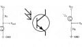
An important implication of Equation 6 is that it suggests a method for generating narrowband angle-modulated waves through the use of analog multipliers and summers. The block diagram for this circuit is shown in Figure 6.

 

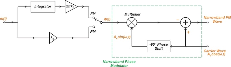
Figure 6. Block diagram of a circuit for generating narrowband angle-modulated signals.

 

In a future article, we’ll see that the above circuit serves as a fundamental building block for generating wideband angle-modulated signals. This is achieved through a process known as narrowband-to-wideband conversion.

 

Wrapping Up

Angle modulation, including phase and frequency modulation, plays a crucial role in communication systems and is also key in analyzing circuits such as oscillators and frequency synthesizers. In this article, we considered a simple message spectrum to gain insight into the spectra produced by narrowband angle modulation. As we learned, these spectra approach twice the message bandwidth. In the next article, we’ll continue this discussion by exploring narrowband modulation of a single-frequency message signal.

 

This article is Part 4 of a ten-part series on angle-modulated signals. All articles in this series are listed below in order of publication:

1. Introduction to Phase Modulation for RF Systems
2. Using Instantaneous Frequency to Represent PM and FM Signals
3. Understanding the Differences Between Phase and Frequency Modulation
4. Introduction to Narrowband Angle Modulation
5. Practical Insights Into Narrowband FM With a Single-Frequency Input
6. Introduction to Wideband FM Signals
7. Exploring Bessel Functions: Understanding the Spectrum of Tone-Modulated FM
8. Three Methods for Estimating the Transmission Bandwidth of FM Signals
9. Exploring the Relationship Between FM Wave Bandwidth and the Modulation Index
10. Estimating FM Wave Bandwidth: Solved Examples

 

​​​​​​​All images used courtesy of Steve Arar