Understanding the Differences Between Phase and Frequency Modulation

Though both frequency modulation (FM) and phase modulation (PM) fall under the umbrella of angle modulation, the waveforms they produce differ. FM’s frequency deviation depends solely on the message signal’s amplitude, whereas PM’s frequency deviation is dependent on both the amplitude and frequency of the message signal. In this article, we’ll enhance our understanding of FM and PM waves by exploring these differences.

 

PM and FM Waves

The PM and FM waves for any message signal can be obtained by Equations 1 and 2, respectively:

$$s_{PM}(t) ~=~ A_c \cos[ 2 \pi f_c t ~+~ k_p m(t) ]$$

Equation 1.

 

$$s_{FM}(t) ~=~ A_c \cos \big [ 2 \pi f_c t ~+~ 2 \pi k_f \int_{0}^{t} m(\alpha) d \alpha \big ]$$

Equation 2.

 

where:

m(t) is the message signal

A_c is the amplitude of the carrier

f_c is the carrier frequency

k_p is the phase deviation constant

k_f is the frequency deviation constant.

 

FM and PM Waves for a Sinusoidal Message

To start with, let’s assume that the message signal is a sinusoidal function given by:

$$m(t) ~=~ A_m \cos ( 2 \pi f_m t)$$

Equation 3.

 

We can readily obtain the PM wave for this message signal by applying Equation 1:

$$s_{PM}(t) ~=~ A_c \cos[ 2 \pi f_c t ~+~ k_p A_m \cos ( 2 \pi f_m t) ]$$

Equation 4.

 

After that, we derive the FM wave by integrating the message signal:

$$s_{FM}(t) ~=~ A_c \cos[ 2 \pi f_c t ~+~ \frac{k_f A_m}{2 \pi f_m} \sin ( 2 \pi f_m t) ]$$

Equation 5.

 

The resulting waveforms can be seen, along with the original message signal, in Figure 1.

 

Figure 1. A sinusoidal message signal (top), the corresponding PM wave (middle), and the corresponding FM wave (bottom).

 

Note that these waveforms use the following parameter values:

f_c = 100 Hz

A_m = 1 V

f_m = 2.5 Hz

k_p = 20 rad\V

k_f = 300 Hz/V.

As we would expect based on the previous article in this series, the frequency of the PM wave rises when m(t) has a positive slope and falls when it has a negative slope. To examine the frequency variations of the FM wave, we need to find its instantaneous frequency:

$$\begin{eqnarray}f_i(t) &~=~& \frac{1}{2 \pi} \frac{d \theta_i}{dt} \\&~=~& \frac{1}{2 \pi} \frac{d}{dt} \big [2 \pi f_c t ~+~ \frac{k_f A_m}{2 \pi f_m} \sin ( 2 \pi f_m t) \big ] \\&~=~& f_c ~+~ \frac{1}{2 \pi} ~\times~ \frac{k_f A_m}{2 \pi f_m} ~\times~ 2 \pi f_m \cos ( 2 \pi f_m t) \\&~=~& f_c ~+~ \frac{k_f A_m}{2 \pi} ~\times~ \cos ( 2 \pi f_m t)\end{eqnarray}$$

Equation 6.

 

where θ_i is the instantaneous angle.

Two observations are in order here. First, while the PM wave’s frequency depends on the slope of m(t), the frequency of the FM wave varies with the instantaneous value of the message signal. Figure 1 corroborates this, showing that the FM wave frequency is at its maximum when the message signal is at its peak value, and at its minimum when the message signal is at its lowest.

Second, Figure 1 illustrates that the PM and FM waves for a sinusoidal message signal can’t be distinguished from each other without seeing the message signal. However, as we’ll see shortly, this isn’t the case for a non-sinusoidal message signal.

 

How Does the Instantaneous Frequency Change with A_m?

Before we get to that, let’s take a closer look at the instantaneous frequency in the above example and see how it varies with the message amplitude (A_m). We obtain the instantaneous frequency of the PM wave by taking the derivative of its instantaneous angle:

$$\begin{eqnarray}f_i(t) &~=~& \frac{1}{2 \pi} \frac{d \theta_i}{dt} \\&~=~& \frac{1}{2 \pi} \frac{d}{dt} \big [2 \pi f_c t ~+~ k_p A_m \cos ( 2 \pi f_m t) \big ] \\&=& f_c ~-~ \frac{1}{2 \pi} ~\times~ k_p A_m ~\times~ 2 \pi f_m \sin ( 2 \pi f_m t) \\&~=~& f_c ~-~ k_p A_m f_m \sin ( 2 \pi f_m t)\end{eqnarray}$$

Equation 7.

 

The message-dependent part of the instantaneous frequency is called the frequency deviation. For the PM wave, it’s given by:

$$f_{d, pm} ~=~ - k_p A_m f_m \sin ( 2 \pi f_m t)$$

Equation 8.

 

Similarly, we can use the instantaneous frequency of the FM wave provided in Equation 6 to determine the frequency deviation of the FM signal:

$$f_{d, fm} ~=~ \frac{k_f A_m}{2 \pi} ~\times~ \cos ( 2 \pi f_m t)$$

Equation 9.

 

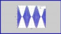
Equations 8 and 9 show that the frequency deviations of both PM and FM waves are proportional to the message signal amplitude (A_m). Figure 2 provides some waveforms to help us better understand this relationship.

 

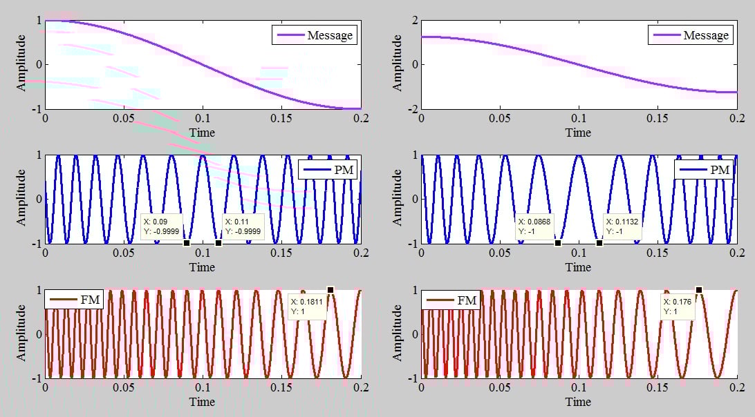
Figure 2. Top: message signals for A_m = 1 V (left) and A_m = 1.25 V (right). Middle: the corresponding PM waves. Bottom: the corresponding FM waves. [click to enlarge]

 

The left-hand column in the above figure displays the waveforms for a message amplitude of A_m = 1 V. The right-hand column displays the waveforms for A_m = 1.25 V. For both sets of waveforms, the following is true:

f_c = 100 Hz

f_m = 2.5 Hz

k_p = 20 rad/V

k_f = 300 Hz/V.

Let’s use the data in Figure 2’s cursor boxes to compare the lowest frequencies produced by the two PM waves. Note that clicking on Figure 2 will open a larger version of the image in a new tab, which you may find helpful for readability.

For A_m = 1 V, Equation 10 allows us to estimate the PM wave’s lowest frequency by identifying the longest period in the waveform:

$$f_{min} \approx \frac{1}{0.11-0.09}~=~ 50 ~\text{Hz} \quad \Rightarrow \quad f_{d1} ~=~ -50 ~\text{Hz}$$

Equation 10.

 

In the above equation, we find the frequency deviation (f_d1) by subtracting f_c = 100 Hz from f_min. Similarly, for A_m = 1.25 V, we have:

$$f_{min} ~\approx~ \frac{1}{0.1132~-~0.0868}~=~ 37.88 ~\text{Hz} \quad \Rightarrow \quad f_{d2} ~=~ -62.12 ~\text{Hz}$$

Equation 11.

 

The ratio of the frequency deviations is:

$$\big | \frac{f_{d2}}{f_{d1}} \big |~=~\frac{62.12}{50}~=~1.24$$

Equation 12.

 

which is close to the ratio of the corresponding message amplitudes (1.25/1 = 1.25). We can therefore conclude that the frequency deviation of the PM wave scales with the message amplitude.

We verify that the frequency deviation of the FM wave is proportional to the message amplitude by following a similar procedure. Using the data points for A_m = 1 V, we again use the longest period of the waveform to estimate the lowest frequency:

$$f_{min} ~\approx~ \frac{1}{0.2~-~0.1811}~=~ 52.91 ~\text{Hz} \quad \Rightarrow \quad f_{d1} ~=~ -47.09 ~\text{Hz}$$

Equation 13.

 

For A_m = 1.25 V, we obtain:

$$f_{min} ~\approx~ \frac{1}{0.2~-~0.176}~=~ 41.67 ~\text{Hz} \quad \Rightarrow \quad f_{d2} ~=~ -58.33 ~\text{Hz}$$

Equation 14.

 

The ratio of f_d2 to f_d1 is about 1.24, which is acceptably close to the expected value of 1.25 (the ratio of A_m = 1.25 V to A_m = 1 V).

 

The Differing Effects of Message Signal Frequency

Examining the frequency deviations of the FM and PM waves (Equations 8 and 9) highlights an important difference between these two modulation schemes. In contrast to the FM wave, the frequency deviation of the PM wave is influenced by the message signal frequency (f_m). To illustrate this, let’s generate the waveforms from the previous section using two different values for f_m:

• f_m = 2.5 Hz
• f_m = 2 Hz.

Keeping the other parameters unchanged, we obtain the waveforms in Figure 3.

 

Figure 3. Message signals (top), PM waves (middle), and FM waves (bottom). Left column: f_m = 2.5 Hz. Right column: f_m = 2 Hz. [Click to enlarge]

 

From Equation 10, the frequency deviation for the PM wave with f_m = 2.5 Hz is f_d1 = –50 Hz. For f_m = 2 Hz, the frequency deviation works out to –39.76 Hz, as calculated below:

$$f_{min} ~\approx~ \frac{1}{0.1333~-~0.1167}~=~ 60.24 ~\text{Hz} \quad \Rightarrow \quad f_{d2} ~=~ -39.76 ~\text{Hz}$$

Equation 15.

 

The ratio of the frequency deviations is:

$$\big | \frac{f_{d2}}{f_{d1}} \big |~=~\frac{39.76}{50}~=~0.8$$

Equation 16.

 

which is the same as the ratio of the message signal frequencies (2/2.5 = 0.8).

The frequency deviation of the FM wave with f_m = 2.5 Hz is f_d1 = –47.09 Hz, as calculated earlier by Equation 13. For f_m = 2 Hz, we obtain:

$$f_{min} ~\approx~ \frac{1}{0.25-0.231}~=~ 52.63 ~\text{Hz} \quad \Rightarrow \quad f_{d2} ~=~ -47.37 ~\text{Hz}$$

Equation 17.

 

This is acceptably close to f_d1 = –47.09 Hz, indicating that the frequency deviation of the FM wave is independent of the message frequency.

 

Summary of Frequency Deviation Variations

Before we continue, let’s take a moment to summarize what we’ve learned. In both FM and PM, the frequency deviation is directly proportional to the amplitude of the message signal (A_m). This is illustrated in Figure 4.

 

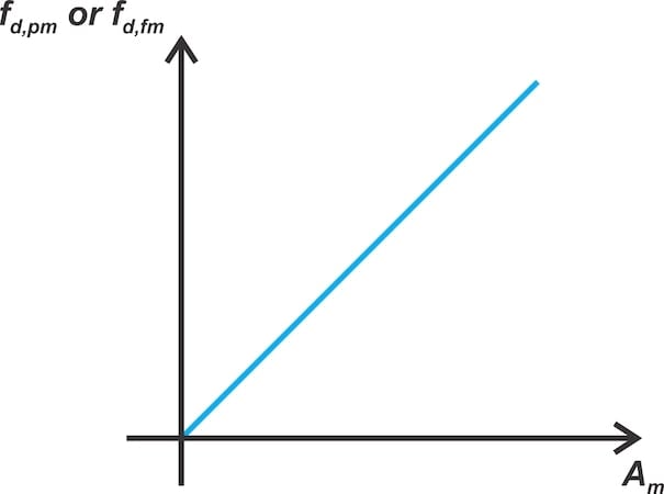
Figure 4. The impact of message amplitude on frequency deviation is the same for both FM and PM waves.

 

The frequency deviation of the PM wave is also directly proportional to the message frequency (f_m). However, the frequency deviation in the FM scheme remains unaffected by f_m. These relationships are depicted in Figure 5.

 

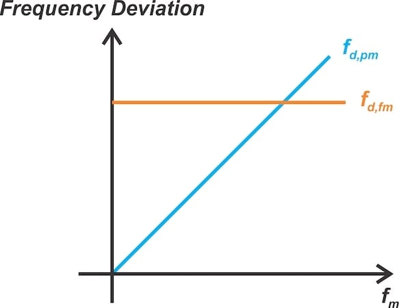
Figure 5. The impact of message frequency on the FM (orange) and PM (blue) waves’ frequency deviation.

 

FM and PM Waveforms for a Step-Function Message

So far, we’ve only discussed the FM and PM waves produced by a sinusoidal message signal. But what if the message signal is a step function? Figure 6 shows the waveforms for this example.

 

Figure 6. A step-function message signal (top), the corresponding PM wave (middle), and the corresponding FM wave (bottom).

 

The message function in Figure 6 incorporates a unit step change at t = 0.05 seconds, transitioning from 0 to 1. For t < 0.05 seconds, the message signal is zero, and we have an unmodulated carrier wave. For t > 0.05 seconds, m(t) has a constant value of unity.

The middle portion of the figure shows the PM wave corresponding to this message signal. With k_p = π/2, the PM scheme introduces an abrupt phase shift of π/2. As we learned in an earlier article on phase modulation, a constant message signal introduces a phase shift without altering the frequency of the PM wave. Consequently, the PM wave’s frequency remains the same after the step function transition.

To determine the FM wave, note that the integral of a unit step function grows linearly with time, maintaining a slope of unity. This introduces a term (2πk_ft) to the argument of the carrier wave. Therefore, for t > 0.05 seconds, we can express the FM wave as:

$$\begin{eqnarray}s_{FM}(t) &~=~& A_c \cos \big [ 2 \pi f_c t ~+~ 2 \pi k_f \int_{0}^{t} m(\alpha) d \alpha \big ] \\&~=~& A_c \cos \big [ 2 \pi f_c t ~+~ 2 \pi k_f t \big ]\end{eqnarray}$$

Equation 18.

 

This shows that the frequency of the FM wave increases by k_f after the step function transition.

Contrast the angle-modulated waveforms in Figure 1, where we used a sinusoidal message signal, with those in Figure 6. In Figure 1, it would be impossible to distinguish the PM waveform from the FM waveform if the message signal weren’t displayed. However, this is not the case in Figure 6. Depending on the type of message signal, PM and FM schemes can result in either similar or completely different waveforms.

 

Wrapping Up

In amplitude modulation, the envelope of the modulated wave directly mirrors the changes in the message signal. In angle modulation, the influence of the message signal on the carrier wave is more subtle. However, the details of this relationship differ depending on the type of angle modulation.

One major difference lies in how the frequency deviation relates to the message signal. In FM, the frequency deviation is solely influenced by the message signal’s amplitude. By contrast, PM’s frequency deviation is affected by both the amplitude and frequency of the message signal. I hope the examples in this article have helped you understand how the message signal affects both types of angle-modulated waves.

 

This article is Part 3 of a ten-part series on angle-modulated signals. All articles in this series are listed below in order of publication:

1. Introduction to Phase Modulation for RF Systems
2. Using Instantaneous Frequency to Represent PM and FM Signals
3. Understanding the Differences Between Phase and Frequency Modulation
4. Introduction to Narrowband Angle Modulation
5. Practical Insights Into Narrowband FM With a Single-Frequency Input
6. Introduction to Wideband FM Signals
7. Exploring Bessel Functions: Understanding the Spectrum of Tone-Modulated FM
8. Three Methods for Estimating the Transmission Bandwidth of FM Signals
9. Exploring the Relationship Between FM Wave Bandwidth and the Modulation Index
10. Estimating FM Wave Bandwidth: Solved Examples

 

All images used courtesy of Steve Arar