Three Methods for Estimating the Transmission Bandwidth of FM Signals

Earlier in this series, we delved into the spectrum of FM waves created by a single-frequency message signal, also known as tone-modulated FM. As we learned, this spectrum consists of an infinite number of sidebands. However, only a finite number of these sidebands contain a significant amount of power. When determining the bandwidth required to transmit a signal, only the significant sidebands need to be taken into account.

But what counts as 'significant' in this context? How we answer that question effectively determines the distortion level we're willing to accept in our design. We can reduce the distortion by accommodating a larger number of spectral components.

In this article, we'll discuss two different ways of defining the effective bandwidth of an FM signal. We'll then learn about Carson's rule, an easy and reasonably accurate estimation method. Though grounded in the analysis of tone-modulated FM waves, these approaches can be used to find the transmission bandwidth of other FM signals as well.

 

Tone-Modulated FM Waves

With an arbitrary modulation index of β, the equation for a tone-modulated FM wave may be written as:

$$s(t) ~=~ A_c \sum_{n = - \infty}^{n = \infty} J_n(\beta) \cos \big [( \omega_c ~+~ n \omega_m)t \big ]$$

Equation 1.

 

where A_c is the amplitude of the carrier wave.

The nth-order sideband component is scaled by the Bessel function of the first kind, J_n(β). Figure 1 shows the typical spectrum of a tone-modulated FM wave for A_c = 1.

 

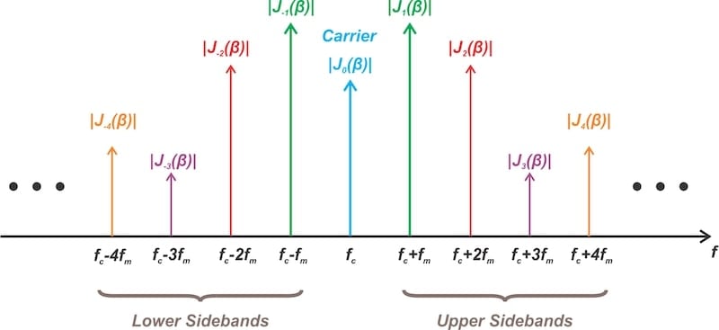
Figure 1. Typical spectrum of an FM signal for a single-tone message signal. Image used courtesy of Steve Arar

 

Strictly speaking, the bandwidth of an FM wave is infinite. This is clear from Equation 1. However, for large n, J_n(β) can be approximated by:

$$J_n( \beta ) ~\approx~ \frac{ \beta ^n}{2^n \ n!}$$

Equation 2.

 

This means that J_n(β) approaches zero for sufficiently large values of n. Therefore, not all sidebands of an FM wave contain significant power.

 

Effective Bandwidth Based on Relative Sideband Amplitudes

One method to define the effective bandwidth of a tone-modulated FM signal is to disregard sidebands with a relative amplitude below a set threshold. In mathematical terms, we define the transmission bandwidth as:

$$BW~=~2n_{max}f_m$$

Equation 3.

 

where:

f_m is the frequency of the message signal

n_max represents the highest integer index at which |J_n(β)| exceeds a defined threshold.

In Equation 3, we multiply 2n_max by f_m because the spectral components are spaced by f_m (see Figure 1). The value of n_max for a given β can be easily determined from tabulated values of J_n(β). By way of example, consider J_n(β) for β = 2 and the various values of n shown in Table 1.

 

Table 1. J_n(β) for β = 2 and various values of n.

n	0	1	2	3	4	5	6
Jn(β)	0.224	0.577	0.353	0.129	0.034	0.007	0.001

 

Let's say we set the threshold at 1% of the unmodulated carrier. The highest value of n that satisfies |J_n(β)| > 0.01 is n_max = 4, leading to an effective bandwidth of BW = 8f_m for β = 2.

Alternatively, we could use 1% as the threshold for significance. Figure 2 shows n_max as a continuous function of β for both the 1% and 10% criteria.

 

Figure 2. The number of significant sideband pairs as a function of β. Image used courtesy of A. B. Carlson

 

The bandwidth for a 1% threshold is often excessively conservative. On the other hand, the 10% threshold causes small yet noticeable distortion. For most applications, n_max values between these two limits are generally appropriate.

In some cases, the effective bandwidth for a specific threshold is provided as a plot of BW/Δf versus β. Figure 3 shows such a plot for the 1% threshold.

 

Figure 3. Plot of bandwidth normalized to the frequency deviation (BW/Δf) versus β. Image used courtesy of Simon Haykin

 

Power-Based Approach to Defining the Effective Bandwidth

We can also define the effective bandwidth as the frequency range that contains a specific proportion of the total power. For example, the distortion is often deemed tolerable if the chosen bandwidth captures 98% or more of the FM wave's power.

Let's use the data in Table 1 to determine the bandwidth that captures 98% or more of the FM wave's power for β = 2. The power of the FM wave with N sidebands is:

$$P_N~=~ \frac{1}{2} \ A_c^2 \ \sum_{n=- N}^{N} J_n^2( \beta)$$

Equation 4.

 

The total power of the FM wave is given by:

$$P_{tot}~=~ \frac{1}{2} \ A_c^2$$

Equation 5.

 

We want to determine the smallest value of N that satisfies:

$$P_N ~\ge~ 0.98 ~\times~ P_{tot} ~\rightarrow~ \sum_{n=- N}^{N} J_n^2( \beta) ~\ge~ 0.98$$

Equation 6.

 

Substituting the data in Table 1 and applying the property |J_-n(β)| = |J_n(β)|, we have:

$$J_0^2(2) ~+~ 2J_1^2(2) ~+~ 2J_2^2(2) ~+~ \ldots ~+~ 2J_N^2(2) ~\ge~ 0.98$$

Equation 7.

 

The smallest value of N that satisfies the above equation is N = 3, leading to an effective bandwidth of BW = 6f_m for β = 2.

 

Carson's Rule

Interestingly, if we consider the bandwidth for 98% or more of the FM wave's power for different values of β, we find that the number of significant sidebands is always N = β + 1. This is known as Carson's rule.

According to Carson's rule, the transmission bandwidth that includes 98% or more of a tone-modulated FM wave's power is:

$$BW ~=~ 2(\beta ~+~1) f_m$$

Equation 8.

 

The above equation can also be written as:

$$BW ~=~ 2(\Delta f ~+~ f_m)$$

Equation 9.

 

where Δf is the maximum frequency deviation. Note that Equations 8 and 9 are also applicable for β ≪ 1. In that case, we have a narrowband FM wave with a bandwidth of BW ≈ 2f_m.

 

Example 1: Determining the Bandwidth of FM Waves

Consider a 2 kHz carrier that is frequency-modulated by a 150 Hz sinusoidal signal. The peak frequency deviation (Δf) is 20 Hz. What is the approximate bandwidth of this FM wave? With f_m = 150 Hz and Δf = 20 Hz, we have:

$$\beta ~=~ \frac{\Delta f}{f_m} ~=~ \frac{20}{150}~=~0.133$$

Equation 10.

 

This is a narrowband FM signal. Applying Carson's rule, we obtain the bandwidth:

$$BW ~\approx~ 2(\Delta f ~+~ f_m)~=~2 (20 ~+~ 150)~=~340 \ \text{Hz}$$

Equation 11.

 

This is close to the expected value of 2f_m = 300 Hz from our narrowband FM analysis.

Figure 4 illustrates the spectrum of the modulated signal near the carrier frequency, obtained by performing a fast Fourier transform (FFT) on the signal.

 

Figure 4. The spectrum of the tone-modulated FM wave for Δf = 20 Hz, f_m = 150 Hz and β = 0.133. Image used courtesy of Steve Arar

 

Note that the amplitude of the sideband component in the cursor box agrees with the value of J₁(0.133) = 0.0665.

Let's repeat this exercise with f_m = 2 Hz and Δf = 50 Hz. What would the bandwidth be then?

With f_m = 2 Hz and Δf = 50 Hz, we have β = 25. Applying Carson's rule, the bandwidth is estimated as:

$$BW ~\approx~ 2(\Delta f ~+~ f_m)~=~2 (50 ~+~ 2)~=~104 \ \text{Hz}$$

Equation 12.

 

The simulated output spectrum for this case is displayed in Figure 5, which shows a bandwidth consistent with Carson's rule.

 

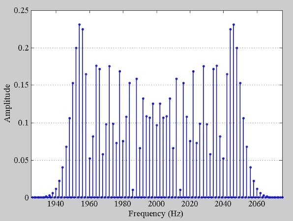
Figure 5. The spectrum of the tone-modulated FM wave for Δf = 50 Hz, f_m = 2 Hz, and β = 25. Image used courtesy of Steve Arar

 

FM Bandwidth For an Arbitrary Message Signal

In the above discussion, we verified Carson's rule for a tone-modulated FM signal using the table of Bessel functions. A tone-modulated FM wave doesn't accurately reflect real-world scenarios. Usually, the message signal comprises a variety of frequencies.

There are no straightforward expressions for determining the FM spectrum for an arbitrary message signal. When determining the FM wave's bandwidth, however, it's possible to generalize the results of the tone-modulated FM analysis to non-sinusoidal modulating signals. In this case, we define the deviation ratio (D) as the maximum frequency deviation (Δf) divided by the maximum modulating frequency (W) present in the message signal:

$$D ~=~ \frac{\Delta f}{W}$$

Equation 13.

 

The deviation ratio is analogous to the modulation index of tone modulation. Replacing β with D, we can determine the number of significant sideband components (n_max) and estimate the required bandwidth using the following equation:

$$BW ~=~ 2 n_{max}W$$

Equation 14.

 

In this case, we know that n_max is dependent on D. Rather than using curves and tables to determine n_max, we can apply Carson's rule by replacing β with D and f_m with W:

$$BW ~=~ 2 (\Delta f ~+~ W) ~=~ 2(D~+~1)W$$

Equation 15.

 

In fact, we commonly use Carson's rule as a convenient way to estimate the FM bandwidth when working with general modulating signals that are band-limited and possess finite power.

 

Example 2: Bandwidth of Broadcast FM Stations

The Federal Communications Commission (FCC) allows a frequency deviation of Δf = 75 kHz for commercial FM broadcasting. The highest audio frequency is commonly assumed to be W = 15 kHz, leading to a deviation ratio of:

$$D~=~\frac{\Delta f}{W}~=~\frac{75}{15}~=~5$$

Equation 16.

 

Applying Carson's rule, the FM signal bandwidth is:

$$BW ~=~ 2(D~+~1)W ~=~ 2(5~+~1) ~\times~ 15 \ \text{kHz} ~=~180 \ \text{kHz}$$

Equation 17.

 

In practice, broadcast FM channels are 200 kHz wide, which is slightly greater than the value estimated above. The purpose of this is to reduce the selectivity requirements of receivers.

 

Wrapping Up

The number of significant sidebands for the FM wave transmission depends on the intended application and the fidelity requirements. There are several methods for determining the bandwidth needed for FM wave transmission. In particular, Carson's rule is a convenient estimation method that offers reasonable accuracy.

 

This article is Part 8 of a ten-part series on angle-modulated signals. All articles in this series are listed below in order of publication:

1. Introduction to Phase Modulation for RF Systems
2. Using Instantaneous Frequency to Represent PM and FM Signals
3. Understanding the Differences Between Phase and Frequency Modulation
4. Introduction to Narrowband Angle Modulation
5. Practical Insights Into Narrowband FM With a Single-Frequency Input
6. Introduction to Wideband FM Signals
7. Exploring Bessel Functions: Understanding the Spectrum of Tone-Modulated FM
8. Three Methods for Estimating the Transmission Bandwidth of FM Signals
9. Exploring the Relationship Between FM Wave Bandwidth and the Modulation Index
10. Estimating FM Wave Bandwidth: Solved Examples