Introduction to Phase Modulation for RF Systems

From communication systems to radio navigation, modulation is essential for a broad range of RF applications. Accordingly, many different forms of RF modulation exist. In an earlier series of articles, for example, we learned about several different amplitude modulation (AM) techniques. Now, in a new series, we’ll examine two more types of continuous-wave modulation:

• Phase modulation (PM), which changes the phase of the carrier in proportion to the message signal.
• Frequency modulation (FM), which changes the time derivative of the carrier’s phase in proportion to the message signal.

Both PM and FM hold the amplitude of the carrier wave constant and use the message signal to alter the angle of the carrier wave. For that reason, they are collectively known as angle modulation techniques. An angle-modulated signal may be defined as:

$$s(t) ~=~ A_c \cos[ \theta_i (t) ]$$

Equation 1.

 

where θ_i is the instantaneous angle of the message signal.

In amplitude modulation, the envelope of the modulated wave clearly mirrors the message signal. In angle modulation, the influence of the message signal on the carrier wave is less obvious. This is particularly true of phase modulation.

In this article, we’ll clarify this relationship by examining how phase modulation affects three different types of input signals. Before we get to that, however, let’s develop a basic understanding of phase modulation.

 

Phase-Modulated Signals

In phase modulation, the instantaneous phase angle (θ_i) varies linearly with the message signal:

$$\theta_i (t)~=~2 \pi f_c t ~+~ k_p m(t)$$

Equation 2.

 

where:

m(t) is the message signal

f_c is the carrier frequency

k_p is a constant.

Let’s see how this PM signal compares to an unmodulated carrier wave with a frequency of f_c and a constant initial phase of ϕ₀, as given by Equation 3.

$$c(t)~=~ A_c \cos[2 \pi f_c t ~+~ \phi_0]$$

Equation 3.

 

The unmodulated carrier wave can be represented by a phasor that rotates at a constant angular velocity of 2πf_c. This is illustrated in Figure 1(a).

 

Figure 1. The phasor representation of an unmodulated signal (a) and a phase-modulated signal (b).

 

What about the PM wave? Assuming that k_pm(t) is significantly less than 2πf_ct, we still have a phasor with amplitude A_c that rotates in a counterclockwise direction. This is illustrated in Figure 1(b).

However, as we know from Equation 2, the instantaneous phase is a function of the message signal. We can view the term 2πf_ct in Equation 2 as the central value of the instantaneous phase. The total phase fluctuates about this central value.

With k_p > 0, positive values of the message signal cause the instantaneous angle (θ_i) to increase above the central value, while negative values of m(t) bring the instantaneous phase below the central value.

 

Phase-Modulating a Sinusoidal Wave

For our first example, let’s assume that the following message signal:

$$m(t) ~=~ \cos(2 \pi ~\times~ 2.5 ~\times~ t)$$

Equation 4.

 

is used to phase-modulate a 20 Hz carrier. With k_p = 0.5 rad/V, the modulated wave is:

$$s_{PM}(t) ~=~ \cos \big [ 2 \pi ~\times~ 20 ~\times~ t ~+~ 0.5~\times~ \cos(2 \pi ~\times~ 2.5 ~\times~ t) \big ]$$

Equation 5.

 

These waveforms are plotted in Figure 2.

 

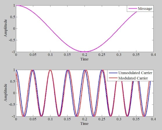
Figure 2. Top plot: the message signal. Bottom plot: the unmodulated carrier (blue) and phase-modulated signal (red). Note that phase modulation changes the zero crossings of the carrier.

 

Unlike in amplitude modulation schemes, the amplitude of the PM wave doesn’t change with the message signal. With PM modulation, the message information is contained in the zero crossings of the modulated wave. The unmodulated wave's zero-crossing points are evenly spaced in time.

When the message signal approaches zero—for instance, around t = 0.1 seconds—the modulated wave matches the unmodulated carrier. However, the zero crossings of the modulated wave are not periodic. For non-zero values of m(t), the modulated wave may lead or lag the carrier, resulting in a phase difference.

 

Phase-Modulating a Ramp Signal

As our next example, let’s say that the magenta curve in Figure 3 is our message signal. This signal is a ramp that rises to unity at a slope of 2 and then falls back to zero at a slope of –2.

 

Figure 3. Using a ramp as the modulating signal (top) to produce a PM wave (bottom).

 

If we use this ramp input with k_p = 10π rad/V to phase-modulate a 20 Hz carrier, we obtain the waveform in the lower half of Figure 3. In this case, phase modulation manifests itself as a change in the frequency of the waveform. To understand why, let’s consider the rising and falling portions of the message signal separately.

 

The Rising Signal

The rising part of the message signal in Figure 3 can be described by m(t) = 2t. The modulated wave for this portion of the message signal is:

$$\begin{eqnarray}s_{PM}(t) &~=~& \cos ( 2 \pi ~\times~ 20 ~\times~ t ~+~ 10 \pi ~\times~ 2t ) \\&~=~& cos ( 2 \pi ~\times~ 30 ~\times~ t )\end{eqnarray}$$

Equation 6.

 

Equation 6 shows that the frequency of the modulated signal increases from its center value of 20 Hz to 30 Hz during the rising portion of the ramp input. Note that if we increase the slope of the rising section, we’ll achieve a higher output frequency. For instance, if we use a slope of 4 rather than 2 in Equation 6, the output frequency becomes 40 Hz.

 

The Falling Signal

To simplify our equations for the falling part of the message signal, let’s assume that the time origin is moved to t = 0.5 seconds. As a result, the message signal can be expressed as:

$$m(t) ~=~ 1~-~2t$$

Equation 7.

 

which leads to the following modulated signal:

$$\begin{eqnarray}s_{PM}(t) &~=~& \cos \big [ 2 \pi ~\times~ 20 ~\times~ t ~+~ 10 \pi ~\times~ (1~-~2t ) \big ] \\&~=~& \cos ( 2 \pi ~\times~ 10 ~\times~ t )\end{eqnarray}$$

Equation 8.

 

During the falling part of the message waveform, the frequency of the modulated signal decreases from its center value of 20 Hz to 10 Hz. Figure 3 demonstrates that phase modulation can alter the frequency of the modulated waveform. This shows the close relationship between phase modulation and frequency modulation.

 

Phase-Modulating a Signal with Intervals of Constancy

For our third and final example, let’s use the message signal in Figure 4 to phase-modulate our 20 Hz carrier. This signal is constant from 0.2 to 0.8 seconds.

 

Figure 4. Top plot: a message signal that first ramps up to unity, stays constant for an interval, and finally ramps down to zero. Bottom plot: the corresponding PM wave.

 

We know from our earlier discussion that the output frequency increases when the message signal rises at a constant slope and falls when the message signal decreases at a constant slope. But what about the interval where the message signal remains unchanged?

From the modulated waveform provided in the bottom portion of Figure 4, it’s evident that the PM wave is a sinusoidal signal with a period of 0.05 seconds. We know this because the interval from 0.2 to 0.3 seconds contains two periods of the PM wave.

A period of 0.05 seconds corresponds to a frequency of 20 Hz. Therefore, when the message signal remains constant, the frequency of the modulated wave becomes equal to that of the unmodulated carrier. To verify this mathematically, let’s substitute m(t) = 1 and k_p = 10π into the equation of the modulated wave:

$$\begin{eqnarray}s_{PM} &~=~& \cos \big [ 2 \pi f_c t ~+~ k_p m(t) \big ] \\&~=~& \cos \big [ 2 \pi f_c t ~+~ 10 \pi ~\times~ 1 \big ] \\&~=~& \cos [ 2 \pi f_c t \big ]\end{eqnarray}$$

Equation 9.

 

A constant message signal results in a constant phase shift, causing the frequency of the PM wave to revert to its central value.

 

Test Your Knowledge: Another Sinusoidal Message Signal

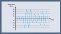
After checking out the waveforms above, you're practically a PM pro! Let's use the sinusoidal message signal in Figure 5 to see how well you know your stuff.

 

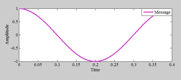
Figure 5. A sinusoidal message signal for generating a PM wave.

 

We know that phase modulation may show up as a change in the frequency of the modulated signal. Which segments of the waveform above will result in the highest output frequencies, and which the lowest?

Figure 6 shows the PM wave obtained by modulating an 80 Hz carrier signal with k_p = 25 rad/V.

 

Figure 6. The message signal (top) and the corresponding PM wave (bottom).

 

Note the cursor box at the bottom left of the figure. By considering this data point, we observe that half the period of the first cycle is about 0.0068 seconds. This corresponds to a frequency of about 73.5 Hz, which is close to the frequency of the unmodulated carrier (f_c = 80 Hz). Therefore, around the message waveform’s peak, the PM wave exhibits a frequency close to the unmodulated carrier.

To understand this, note that the peak of the sinusoidal wave has a very small slope (almost zero). The output frequency is therefore f_c, just as was the case for the flat regions of the message waveform in Figure 4.

Conversely, the descending part of the sinusoidal wave shows its steepest negative slope when it crosses zero around t = 0.1 seconds. This region generates the lowest output frequency. Around t = 0.2 seconds, the slope of the message waveform again approaches zero, producing an output frequency almost equal to the unmodulated carrier frequency.

Finally, as the rising part of the waveform crosses the zero level, it reaches its steepest positive slope, resulting in the maximum output frequency. This is clearly illustrated in Figure 7, which offers a close-up view of the relevant region.

 

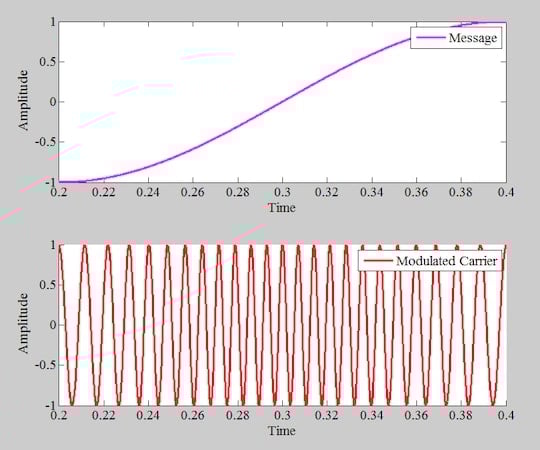
Figure 7. The ascending part of the message signal (top) and the corresponding PM wave (bottom) during the rising part of the message waveform.

 

Wrapping Up

In amplitude modulation, the envelope of the modulated wave mirrors the changes in the message signal. In phase modulation (and, to a lesser extent, frequency modulation), the relationship between the message and carrier waves can be more obscure. For that reason, we began our discussion of phase modulation by observing its effect on several example waveforms. Now that we better understand this tricky relationship, the next article in this series will examine PM and FM from a mathematical perspective.

 

This article is Part 1 in a ten-part series on angle-modulated signals. All articles in this series are listed below in order of publication:

1. Introduction to Phase Modulation for RF Systems
2. Using Instantaneous Frequency to Represent PM and FM Signals
3. Understanding the Differences Between Phase and Frequency Modulation
4. Introduction to Narrowband Angle Modulation
5. Practical Insights Into Narrowband FM With a Single-Frequency Input
6. Introduction to Wideband FM Signals
7. Exploring Bessel Functions: Understanding the Spectrum of Tone-Modulated FM
8. Three Methods for Estimating the Transmission Bandwidth of FM Signals
9. Exploring the Relationship Between FM Wave Bandwidth and the Modulation Index
10. Estimating FM Wave Bandwidth: Solved Examples

 

All images used courtesy of Steve Arar