Practical Insights Into Narrowband FM With a Single-Frequency Input

The previous article in this series introduced us to narrowband angle modulation: frequency modulation (FM) and phase modulation (PM) characterized by a low modulation index. In this article, we’ll delve into narrowband angle modulation with a single-frequency modulating input. Due to its better noise performance, we’ll mostly focus on FM. Once we’ve concluded that portion of our discussion, however, we’ll also spend some time on narrowband PM in the form of phase noise.

 

A Review of Narrowband Angle-Modulated Signals

Let’s start by reviewing what we learned in the preceding articles. An angle-modulated signal with a constant amplitude can be expressed by the following equation:

$$s(t) ~=~ A_c \cos( 2 \pi f_c t ~+~ \phi(t) )$$

Equation 1.

 

where:

A_c is the carrier amplitude

f_c is the carrier frequency

t is the time

ϕ(t) is the phase deviation.

Equations 2 and 3 show the relationship between ϕ(t) and the message signal in PM and FM schemes, respectively:

$$\phi (t) ~=~ k_p m(t)$$

Equation 2.

 

$$\phi (t) ~=~ 2 \pi k_f \int_{0}^{t} m(\tau) \ d \tau$$

Equation 3.

 

where:

m(t) is the message signal

k_p is the proportionality constant

k_f is the phase deviation constant.

Narrowband FM refers to the special case of |ϕ(t)| being much smaller than 1 radian. In this case, Equation 1 can be approximated as:

$$s(t) ~\approx~ A_c \cos( 2 \pi f_c t) ~-~ A_c \phi(t) \sin(2 \pi f_c t)$$

Equation 4.

 

As we learned in the previous article, narrowband PM and FM schemes occupy a maximum bandwidth of twice the message bandwidth. This is also true of double-sideband amplitude modulation (AM) schemes.

 

Narrowband FM for a Single-Frequency Modulating Input

Consider the narrowband FM wave corresponding to the following message signal:

$$m(t)~=~A_m \cos(2 \pi f_m t)$$

Equation 5.

 

Applying Equation 3, ϕ(t) is found to be:

$$\phi(t) ~=~ \frac{k_f A_m}{ f_m} \sin( 2 \pi f_m t)$$

Equation 6.

 

By combining Equations 4 and 6, we obtain the modulated signal:

$$s(t) ~\approx~ A_c \cos( 2 \pi f_c t) ~-~ \frac{k_f A_m A_c}{ f_m} \sin( 2 \pi f_m t) \sin(2 \pi f_c t)$$

Equation 7.

 

which, using a standard trigonometric identity, can be rewritten as:

$$s(t) ~\approx~ A_c \cos( 2 \pi f_c t) ~+~ \frac{k_f A_m A_c}{2 f_m} \Big [ \cos \big ( 2 \pi (f_c~+~f_m) t \big ) ~-~ \cos \big (2 \pi (f_c ~-~ f_m) t \big ) \Big ]$$

Equation 8.

 

The first term in the above equation produces two impulses at ±f_c, which means that the carrier is present at the output spectrum. The terms inside the square brackets produce impulses at all of the following frequencies:

• f_c + f_m
• –(f_c + f_m)
• f_c – f_m
• –(f_c – f_m)

The output spectrum is shown in Figure 1(b).

 

Figure 1. The spectra of the single-frequency modulating input (a) and the corresponding narrowband FM signal (b).

 

Narrowband FM vs. Conventional AM

Let’s see how the above spectrum compares to that of a conventional AM signal. Recall that conventional AM is generated using the following equation:

$$s_{AM}(t) ~=~ A_c \Big ( 1~+~ \mu m(t) \Big ) \cos(\omega_c t)$$

Equation 9.

 

You can easily verify that the conventional AM wave corresponding to m(t) = A_mcos(2πf_mt) has the spectrum shown in Figure 2(b).

 

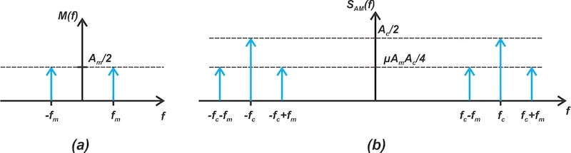
Figure 2. The spectra of the single-frequency modulating input (a) and the corresponding conventional AM signal (b).

 

Comparing Figures 1 and 2, we see that both narrowband FM and conventional AM create the same frequency components. However, the phase relationship between these components is different. With FM, the phase sign of the lower sideband at ±(f_c – f_m) is reversed relative to the upper sideband.

To better understand this, let’s compare the phasor diagrams for the two modulation schemes. Figure 3(a) shows the phasor diagram of the three frequency components produced by conventional AM; Figure 3(b) provides the same for narrowband FM.

 

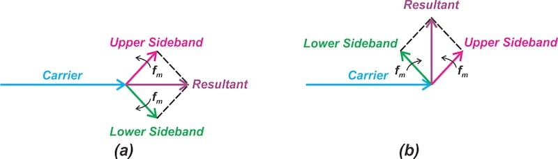
Figure 3. Phasor diagrams for conventional AM (a) and narrowband FM (b) schemes.

 

In both AM and narrowband FM, the sideband phasors rotate in opposite directions at the rate of the message signal frequency. In AM, the sidebands rotate in such a way that the resultant vector always aligns with the carrier. Consequently, the presence of the sidebands only varies the amplitude of the modulated signal.

With narrowband FM, however, the sum of the two sideband vectors produces a vector perpendicular to the carrier wave. This perpendicular component creates frequency (and phase) modulation rather than amplitude modulation.

As a final note, one might argue based on Figure 3 that the amplitude of the overall FM signal isn’t constant. According to the phasor diagram, the rotation of the FM sideband vectors causes changes in the amplitude of the resultant vector and thus in the overall FM signal. In fact, this apparent contradiction arises from the approximations we made to derive Equation 4. Without any approximations, the amplitude of the total vector sum would be exactly constant.

 

Example: Combined FM and AM Modulation

Occasionally, when aiming for AM modulation, circuit imperfections can lead to a mix of narrowband FM and AM. This appears on the spectrum analyzer as two sidebands with unequal amplitude. Because the lower sidebands of the AM and narrowband FM have opposite signs, the lower sideband will have the smaller amplitude. An output spectrum of this type is shown in Figure 4.

 

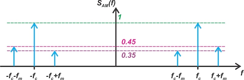
Figure 4. Unequal sidebands arising from the combined influence of narrowband FM and AM.

 

Using what we’ve learned so far, let’s find the modulation index (μ) of the AM signal. We’ll assume that this spectrum was generated from a single-frequency input of m(t) = cos(2πf_mt).

We won't delve into the mathematical details, but with some approximations, we can also assume that both the sidebands of narrowband FM and conventional AM are present at the same time. Using the information provided in Figures 1 and 2, we obtain the amplitude of the combined lower sidebands:

$$\frac{\mu A_m A_c}{4}~-~\frac{k_f A_m A_c}{4f_m}~=~0.35$$

Equation 10.

 

Note that the FM sideband is assumed to have a smaller impact because the intended modulation is AM.

For the upper sideband, we have:

$$\frac {\mu A_m A_c}{4}~+~\frac{k_f A_m A_c}{4f_m}~=~0.45$$

Equation 11.

 

By adding Equations 10 and 11 together, we obtain:

$$\frac {\mu A_m A_c}{2}~=~0.8$$

Equation 12.

 

Note that the amplitude of the carrier component is A_c/2 = 1. Furthermore, with the input being m(t) = cos(2πf_mt), we have A_m = 1. Substituting these values into Equation 12 produces an AM modulation index of μ = 0.8, or 80%.

 

Understanding Oscillator Phase Noise

Above, we discussed a case where narrowband FM occurred unintentionally. Before we wrap up the article, let’s learn a bit about unintentional narrowband phase modulation (PM) as well.

This phenomenon, known as phase noise, often happens in circuits like oscillators. Equation 13 describes the output of an ideal oscillator, which is perfectly periodic:

$$v_{osc}(t) ~=~ A_c \cos( \omega_c t)$$

Equation 13.

 

In this ideal scenario, the zero crossings of the waveform occur at exact integer multiples of 2π/ω_c. In reality, however, there are both deterministic and random factors that alter the zero crossings. Deterministic factors include (but are not limited to):

• Temperature fluctuations.
• Variations in supply voltage.
• Physical vibrations.
• Changes in humidity.
• Nearby magnetic fields.

The random factors are the electrical noise sources within the oscillator circuit that perturb the zero crossings. To account for these perturbations, the oscillator equation may be modified to:

$$v_{osc}(t) ~=~ A_c \cos[ \omega_c t ~+~ \phi_n(t)]$$

Equation 14.

 

where ϕ_n(t), termed the phase noise, is a small, random value.

Note that the above equation matches the definition of phase modulation. Assuming that |ϕ_n(t)| is much less than 1 radian, we can apply our insights from the narrowband angle-modulation discussion to the phase noise phenomenon. For instance, considering the close relationship between PM and FM schemes, Equation 14 implies that the frequency of oscillation slightly deviates from its ideal value.

Also, for |ϕ_n(t)| ≪ 1, the spectrum of v_osc(t) comprises an impulse function at f_c and a replica of the spectrum of ϕ_n(t) translated to a center frequency of f_c. Figure 5 provides an illustrative but perhaps unrealistic example, showing how a replica of the spectrum of ϕ_n(t) is translated to a center frequency of f_c.

 

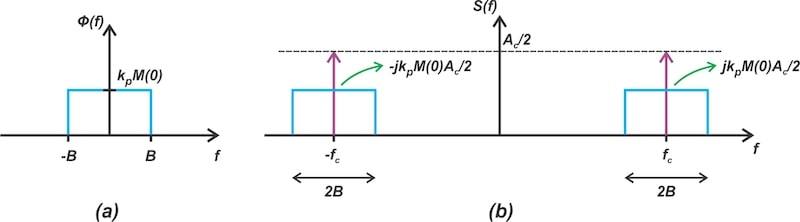
Figure 5. (a) The spectrum of ϕ_n(t) and (b) that of the oscillator’s output.

 

Above, Figure 5(a) above shows the spectrum of ϕ_n(t). Figure 5(b) depicts the spectrum of the oscillator’s output assuming that the narrowband condition is satisfied. A more realistic example of an oscillator spectrum is illustrated in Figure 6.

 

Figure 6. A more realistic example of the oscillator spectrum.

 

Note that the carrier level is not displayed. Instead, the unit dBc is used, indicating that the noise level is normalized relative to the carrier level.

From our previous discussion of narrowband angle modulation, we know that the negative slope in Figure 6 represents the behavior of ϕ_n(t) in the frequency domain. As the above example shows, phase noise tends to be slowly varying, with most of its energy concentrated at low frequencies.

Say that we use a mixer driven by a noisy oscillator, such as the one described by Equation 14, to downconvert an angle-modulated wave. We’ll see that the phase noise of the oscillator directly alters the information component of the output signal. To verify that the phase noise meets the narrowband condition, we can calculate the RMS value of ϕ_n(t) using the measured oscillator spectrum (like that shown in Figure 6). If the RMS value is significantly less than 1 radian, it can be considered narrowband.

 

An Unsolved Example: Using Narrowband FM to Understand Circuit Nonlinearities

In this article, we compared FM and AM modulation of a single-frequency sinusoid. We observed that the angular rotations of the sidebands with respect to the carrier wave are different in AM and narrowband FM. As a final takeaway, I want to present an interesting example from “RF Microelectronics” by B. Razavi for you to solve on your own.

The problem begins with the differential pair in Figure 7. This circuit acts as a hard limiter.

 

Figure 7. A differential pair amplifier acting as a hard limiter, producing one of two possible output levels at any given time.

 

The input applied to the circuit consists of a large sinusoid of amplitude A at f_c and a smaller sinusoid of amplitude a at f_c + f_m. This is illustrated in Figure 8(a).

 

Figure 8. The spectrum of the input applied to the differential pair (a) and the output spectrum (b).

 

Assume that A is large enough to make the differential pair act as a hard limiter, resulting in two distinct output levels at any given time. In other words, A is large enough to steer I_SS completely to one branch of the differential pair at any given time. Explain why the output spectrum should consist of three components at f_c and f_c ± f_m, with sidebands exhibiting opposite signs as shown in Figure 8(b).

Hint: Note that the input can be expressed as a combination of an AM wave and an FM wave. Additionally, consider how a hard limiter responds to each type of AM and FM signals.

 

This article is Part 5 of a ten-part series on angle-modulated signals. All articles in this series are listed below in order of publication:

1. Introduction to Phase Modulation for RF Systems
2. Using Instantaneous Frequency to Represent PM and FM Signals
3. Understanding the Differences Between Phase and Frequency Modulation
4. Introduction to Narrowband Angle Modulation
5. Practical Insights Into Narrowband FM With a Single-Frequency Input
6. Introduction to Wideband FM Signals
7. Exploring Bessel Functions: Understanding the Spectrum of Tone-Modulated FM
8. Three Methods for Estimating the Transmission Bandwidth of FM Signals
9. Exploring the Relationship Between FM Wave Bandwidth and the Modulation Index
10. Estimating FM Wave Bandwidth: Solved Examples

 

All images used courtesy of Steve Arar