 Facebook
 Google
 GitHub
 Linkedin
Understanding Correlation
This article provides insight into the practical aspects of correlation.
This article provides insight into the practical aspects of correlation, specifically the applications of autocorrelation and cross-correlation.
The Meaning of Correlation
In general, correlation describes the mutual relationship which exists between two or more things. The same definition holds good even in the case of signals. That is, correlation between signals indicates the measure up to which the given signal resembles another signal.
In other words, if we want to know how much similarity exists between the signals 1 and 2, then we need to find out the correlation of Signal 1 with respect to Signal 2 or vice versa.
Types of Correlation
Depending on whether the signals considered for correlation are same or different, we have two kinds of correlation: autocorrelation and cross-correlation.
Autocorrelation
This is a type of correlation in which the given signal is correlated with itself, usually the time-shifted version of itself. Mathematical expression for the autocorrelation of continuous time signal x (t) is given by
$$ R_{xx}\left(\tau\right)=\int_{-\infty}^{\infty} x\left(t\right)x^{\star}\left(t-\tau\right) dt $$
where $$ {\star} $$ denotes the complex conjugate.
Similarly the autocorrelation of the discrete time signal x[n] is expressed as
$$ R_{xx}\left[m\right] = \sum_{n=-\infty}^{\infty}x\left[n\right]x^{\star}\left[n-m\right] $$
Next, the autocorrelation of any given signal can also be computed by resorting to graphical technique. The procedure involves sliding the time-shifted version of the given signal upon itself while computing the samples at every interval. That is, if the given signal is digital, then we shift the given signal by one sample every time and overlap it with the original signal. While doing so, for every shift and overlap, we perform multiply and add.
For example, autocorrelation of the digital signal x [n] = {-1, 2, 1} can be computed as shown in Figure 1.
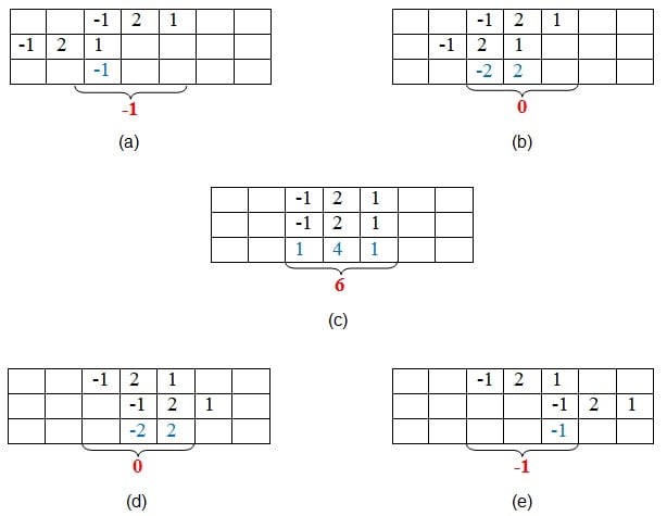
Figure 1: Graphical method of finding autocorrelation
Here, the first set of samples (those in the first row of every table) refers to the given signal. The second set (in the second row of every table) refers to the samples of its time-shifted version. Next, the samples shown in red color in the third row are obtained by multiplying the corresponding samples of the first two rows.
Finally, we add the samples in the last row of the sample (contained within the curly brackets) so as to obtain the samples of the auto-correlated signal.
Thus, here we find that the samples of the autocorrelated signal Rxx are {-1, 0, 6, 0, -1}, where 6 is the zeroth sample.
The example presented shows that the sample of the autocorrelated signal will be at its maximum value when the overlapping signal best matches the given signal. In this case, it happens when time-shift is zero.
Cross-Correlation
This is a kind of correlation, in which the signal in-hand is correlated with another signal so as to know how much resemblance exists between them. Mathematical expression for the cross-correlation of continuous time signals x (t) and y (t) is given by
$$ R_{xy}\left(\tau\right)=\int_{-\infty}^{\infty} x\left(t\right)y^{\star}\left(t-\tau\right) dt $$
Similarly, the cross-correlation of the discrete time signals x [n] and y [n] is expressed as
$$ R_{xy}\left[m\right] = \sum_{n=-\infty}^{\infty}x\left[n\right]y^{\star}\left[n-m\right] $$
Next, just as is the case with autocorrelation, cross-correlation of any two given signals can be found via graphical techniques. Here, one signal is slid upon the other while computing the samples at every interval. That is, in the case of digital signals, one signal is shifted by one sample to the right each time, at which point the sum of the product of the overlapping samples is computed.
For example, cross-correlation of the digital signals x [n] = {-3, 2, -1, 1} and y [n] = {-1, 0, -3, 2} can be computed as shown by Figure 2.
1.jpg)
Figure 2: Graphical method of finding cross-correlation
Here, the first set of samples (in the first row of every table) refers to the signal x [n] and the second set refers to the samples (in the second row of every table) of the signal y [n].
Next, the samples shown in blue color—those in the third row—are obtained by multiplying the corresponding samples of the first two rows. Finally, we add the samples in the last row (contained within the curly brackets) so as to obtain the samples of the cross-correlated signal.
Thus, here we see that the samples of the cross-correlated signal Rxy are obtained as {-6, 13, -8, 8, -5, 1, -1}, where 8 is the zeroth sample.
Further, the example presented shows that the sample of the cross-correlated signal is at its highest peak, with value 13, when the last two samples of y [n] overlap with the first two samples of x [n]. This is because, in this case, the second signal overlaps with the first at its best, as the two samples in each of the signals are identical.
Hence, it can be concluded that the cross-correlation reaches its maximum when the two signals considered become most similar to each other.
Analysis
Now that we've covered the formulation and graphical computation of correlations, let's try to analyze a few cases which reinforce the importance of correlations in practical scenarios.
Case 1: Determining Periodicity
Let us assume that we are asked to determine the periodicity of the received digital signal s [n]. The task can be accomplished by autocorrelating the given signal s [n] with a time-shifted version of itself.
Now, suppose that the result obtained is as shown in Figure 3, wherein the first maximum value of 23 is obtained at time n = 6. Advancing along the time axis, the next maximum is found at n = 12 and is equal to a value of 23 again (our second maximum). Further, the same value of 23 is also found at n = 18 (our third maximum).
This indicates the graph exhibits a value of 23 at regular intervals of 6 (= 12 – 6 and also = 18 – 12) samples. Thus, we can conclude that the given signal has a period of n = 6 samples.
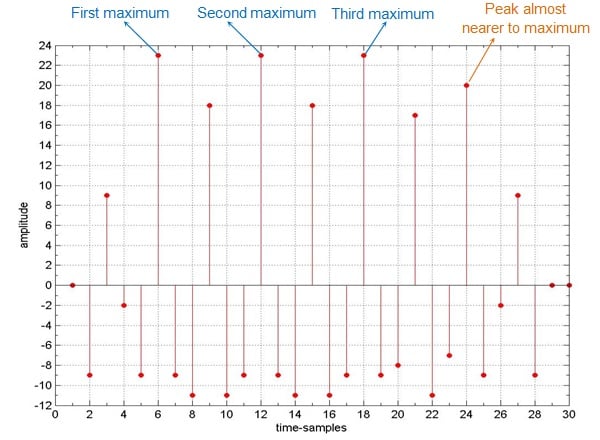
Figure 3: Typical example which shows the use of correlation to find the periodicity of the signal
Given this conclusion, we might expect the next peak to appear at n = 24 (= 18 + 6). However, in the graph, the value at n = 24 is found to be 20 instead of 23. What does this mean!? Does it mean that our first go at analysis was meaningless?
No, not necessarily. Let's analyze.
It is a well-known fact that error is an inevitable part of any system, regardless of whether it's electrical or human. This truth about the errors might be the cause for obtaining a peak-value of 20 at n = 24, instead of the expected value 23.
That is, around the interval of n = 24, the basic repeating signal might have gotten corrupted. Perhaps one or more bit values got changed. Such an error could lead to a slightly lower peak (please note that this can even be the other way round, i.e., slightly higher) than the expected one.
Case 2: Identifying Signal Delays
Let us assume that a signal sent is sent from a transmitter, shown in Figure 4a. The signal arrives at the receiver after being delayed by an unknown interval of time, as shown in Figure 4b.
Now, suppose that we need to find this delay, which is a result of being transmitted over the communication channel. This objective can be achieved by cross-correlating the signal sent with the signal received.
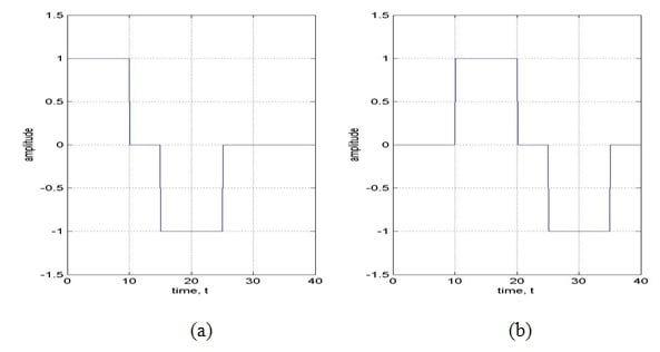
Figure 4: Signal (a) sent and (b) received on a communication channel
The result obtained is shown in Figure 5, which clearly exhibits a peak at time t = 10. This means that the received signal matches with the test signal the best when the test signal is shifted by 10 units along the time-axis.
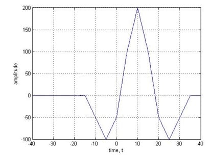
Figure 5: Cross-correlation of the signals shown in Figure 4
Having analyzed the time-shift case, let us now move one more step forward. That is, let us now assume that the received signal has not only been shifted but has also been corrupted by noise.
Figure 6a shows the same signal as that in Figure 4b, but with added noise.
Figure 6b shows the cross-correlation of 6a with the original sent signal from Figure 4a. Here, it is important to note that even this signal exhibits the peak at the same point along the time axis: t = 10.
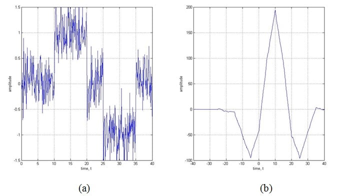
Figure 6: (a) the signal from 4b with noise added and (b) the result of cross-correlating 6a with 4a
Figure 7a shows a much worse case wherein the signal is greatly affected by noise, to the point where it's difficult to make out the shape of the signal with bare eyes. Nevertheless, you can see that the corresponding correlated signal (Figure 7b) exhibits a peak at almost the same point.
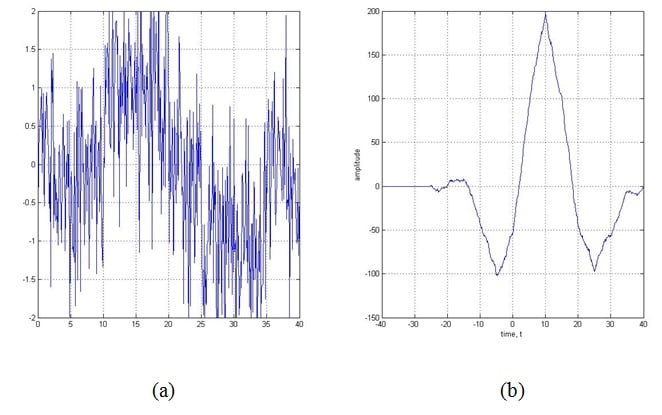
Figure 7: (a) the original signal from 4a shown with a large amount of noise and (b) the correlated signal
Figures 5, 6b, and 7b show that correlation of the signal remains almost the same, even when the signal received is highly corrupted by noise.
Applications
As we've seen in the above examples, correlation is useful in real-world scenarios. There are, in fact, many practical applications for correlation. Here are just a few:
- Signal processing related to human hearing: The human ear interprets signals that are nearly periodic signals to be exactly periodic. This is just like the case where an autocorrelated signal exhibits slightly different maxima-values at regular intervals of time.
- Vocal processing: Correlation can help to determine the tempo or pitch associated with musical signals. The reason is the fact that the autocorrelation can effectively be used to identify repetitive patterns in any given signal.
- Determining synchronization pulses: The synchronization pulses in a received signal, which in turn facilitates the process of data retrieval at the receiver's end. This is because the correlation of the known synchronization pulses with the incoming signal exhibits peaks when the sync pulses are received in it. This point can then be used by the receiver as a point of reference, which makes the system understand that the part of the signal following from then on (until another peak is obtained in the correlated signal indicating the presence of sync pulse) contains data.
- Radar engineering: Correlation can help determine the presence of a target and its range from the radar unit. When a target is present, the signal sent by the radar is scattered by it and bounced back to the transmitter antenna after being highly attenuated and corrupted by noise. If there is no target, then the signal received will be just noise. Now, if we correlate the arriving signal with the signal sent, and if we obtain a peak at a certain point, then we can conclude that a target is present. Moreover, by knowing the time-delay (indicated by the time-instant at which the correlated signal exhibits a peak) between the sent and received signals, we can even determine the distance between the target and the radar.
- Interpreting digital communications through noise: As demonstrated above, correlation can aid in digital communications by retrieving the bits when a received signal is corrupted heavily by noise. Here, the receiver correlates the received signal with two standard signals which indicate the level of '0' and '1', respectively. Now, if the signal highly correlates with the standard signal which indicates the level of '1' more than with the one which represents '0', then it means that the received bit is '1' (or vice versa).
- Impulse response identification: As demonstrated above, cross-correlation of a system's output with its input results in its impulse response, provided the input is zero mean unit variance white Gaussian noise.
- Image processing: Correlation can help eliminate the effects of varying lighting which results in brightness variation of an image. Usually this is achieved by cross-correlating the image with a definite template wherein the considered image is searched for the matching portions when compared to a template (template matching). This is further found to aid the processes like facial recognition, medical imaging, navigation of mobile robots, etc.
- Linear prediction algorithms: In prediction algorithms, correlation can help guess the next sample arriving in order to facilitate the compression of signals.
- Machine learning: Correlation is used in branches of machine learning, such as in pattern recognition based on correlation clustering algorithms. Here, data points are grouped into clusters based on their similarity, which can be obtained by their correlation.
- SONAR: Correlation can be used in applications such as water traffic monitoring. This is based on the fact that the correlation of the signals received by various shells will have different time-delays and thus their distance from the point of reference can be found more easily.
In addition to these, correlation is also exploited to study the effect of noise on the signals, to analyze the fractal patterns, to characterize ultrafast laser pulses, and in many more cases.
Summary
The discussion presented in this article reinforces the fact that the correlation operation is an inevitable part of many signal processing applications.
Related Content


This article makes me think in a current personal project for material characterization , the point is that I need to perform an ultrasonic signal from a transducer and pass it through a physical channel with many points of scattering like the grains in a croncrete block, once I receive the signal in a second ultrasonic transducer maybe a correlation be of great value. ¡There is a lot to learn! but your post was very nice…
Regarding the integral for continuous time autocorrelation, Rxx(τ)=∫∞−∞x(τ)x⋆(t−τ)dt, I wonder if the first term inside the integral should be x(t), not x(tau). If it is x(tau) then that term, x(tau) is a constant, given that the integration is with respect to t, and thus x(tau) can be moved outside the integral. When I compare it to the discrete time version of autocorrelation, which does have the variable in both terms under the sigma, it makes me wonder.