Finding Statistical Relationships with Correlation Coefficients

This series, authored by AAC's Director of Engineering Robert Keim, explores how electrical engineers use statistics. If you're just joining the discussion, you may want to review the previous articles in the series. 

1. Introduction to statistical analysis for EEs
2. Introduction to descriptive statistics for EEs
3. Average deviation, standard deviation, and variance in signal processing
4. Sample size compensation in standard deviation calculations
5. Introduction to the normal/Gaussian distribution
6. Normal distribution: understanding histograms and probability
7. The cumulative distribution function in normally distributed data
8. Understanding parametric tests, skewness, and kurtosis
9. Statistical relationships: correlation, causation, and covariance

 

A Brief Review of Covariance, Correlation, and Causation

In the previous article, we discussed covariance, correlation, and causation.

• Variance quantifies the power of the random deviations in a data set.
• Covariance quantifies a relationship between deviations in two separate data sets. More specifically, it captures the tendency of the values in two data sets to vary together (that is, to co-vary) in a linear fashion.
• Covariance measures the correlation of two variables.
• Correlation does not prove causation—if two variables are correlated, we cannot automatically conclude that changes in one variable cause changes in the other variable. Nonetheless, if we suspect causation and can demonstrate correlation, we have good reason to further investigate the possibility of causation by gathering more data or performing new experiments.

 

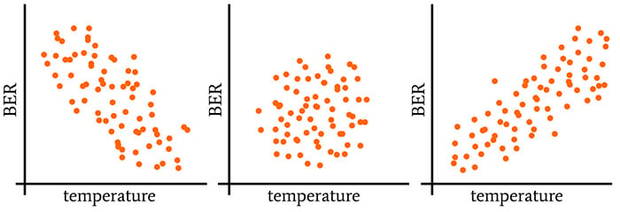
Examples, taken from the previous article, of negative correlation (left), lack of correlation (center), and positive correlation (right). BER stands for bit error rate.

 

Interpreting Covariance

For two data sets with sample size N, we calculate covariance as follows:

 

\[\operatorname {cov} (X,Y)=\frac{1}{N-1}\sum_{i=1}^{N}(X_i-\operatorname {E}[X])(Y_i-\operatorname {E}[Y])\]

 

(The previous article provides an explanation of this formula, if you find it a bit confusing.) Let’s think for a moment about what would happen if we calculated the covariance between a data set and itself:

 

\[\operatorname {cov} (X,X)=\frac{1}{N-1}\sum_{i=1}^{N}(X_i-\operatorname {E}[X])(E_i-\operatorname {E}[X])=\frac{1}{N-1}\sum_{i=1}^{N}(X_i-\operatorname {E}[X])^2\]

 

The formula for covariance has become the formula for variance. Since a data set is perfectly correlated with itself, we see that there is a connection between variance and the maximum possible value of covariance.

This connection extends to standard deviation because variance is equal to standard deviation squared. Thus, the covariance between a data set and itself is equal to the standard deviation squared, i.e., SD(X)SD(X).

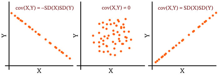
If we extend this to the general case in which we’re calculating the covariance of two different data sets, we can say that perfect linear correlation (and hence maximum covariance) corresponds to a covariance value that is equal to the standard deviation of the first data set multiplied by the standard deviation of the second data set:

 

\[\operatorname {cov} (X,Y)_{MAX}=\operatorname {SD} (X)\operatorname {SD} (Y)\]

 

The same logic applies to two data sets that exhibit perfect inverse correlation. Thus,

 

\[\operatorname {cov} (X,Y)_{MIN}=-\operatorname {SD} (X)\operatorname {SD} (Y)\]

 

Now we have the information we need to interpret covariance values. The covariance range extends from –SD(X)SD(Y), which indicates perfect inverse linear correlation, to +SD(X)SD(Y), which indicates perfect linear correlation. In the middle of this range is zero, which indicates a complete absence of linear correlation.

 

 

Pearson’s Correlation Coefficient

Now we can see why covariance is, from a practical perspective, highly inconvenient. A given degree of correlation can correspond to vastly different covariance values, because the covariance range is determined by the standard deviations of the two data sets.

Thus, we can’t simply report covariance and expect our colleagues to understand the significance of our analysis. We have to report covariance and standard deviations, and the most sensible way to do this is to incorporate the standard deviations into the correlation analysis. This is what we call Pearson’s correlation coefficient:

 

\[\rho_{X,Y}=\frac{\operatorname{cov}(X,Y)}{SD(X)SD(Y)}\]

 

where ρ_X,Y is the Pearson correlation coefficient for the variables X and Y (ρ is lowercase Greek rho). You can see that we’ve simply applied the time-honored technique of normalization.

When we divide the covariance by the product of the two standard deviations, we normalize covariance such that every pair of data sets will produce a value in the range [–1, +1]. The result is a measure of linear correlation that is easily interpreted and that allows for direct comparisons.

As is often the case in statistics, we need to make a distinction between a population and a sample. The symbol ρ denotes the Pearson correlation coefficient of a population. When we’re calculating the Pearson correlation of a sample, we use the letter r:

 

\[r_{xy}={\frac {\sum _{i=1}^{N}(x_{i}-{\bar {x}})(y_{i}-{\bar {y}})}{{\sqrt {\sum _{i=1}^{N}(x_{i}-{\bar {x}})^{2}}}{\sqrt {\sum _{i=1}^{N}(y_{i}-{\bar {y}})^{2}}}}}\]

 

Note that the 1/(N-1) terms cancel out. Also, you may not be familiar with the horizontal bar over X and Y: this is yet another method of denoting a mean, and it is used specifically for the mean of a sample rather than a population. The symbol μ denotes the population mean.

 

Spearman’s Correlation

As you may have read in a previous article, some statistical tests—called parametric tests—can be applied only to data that exhibit a sufficiently normal distribution. Pearson’s correlation coefficient is a parametric test, and consequently, if your data are not sufficiently normal, you need to consider a nonparametric alternative.

The nonparametric version of Pearson’s correlation coefficient is called Spearman’s rank correlation coefficient. The formula is the same, but it’s applied to rank variables and quantifies monotonic correlation instead of linear correlation.

 

Conclusion

Pearson’s correlation coefficient is a valuable and widely-used statistical measure that helps to reveal meaningful and potentially causal relationships between variables. It’s essential for empirical research, and it may even come in handy someday when you’re troubleshooting an electronic system.