Introduction to Normal Distribution in Electrical Engineering

This article is a continuation of our series on statistics in electrical engineering. The first two articles laid the groundwork of our discussion, addressing statistical analysis and descriptive statistics.

We then delved into average deviation, standard deviation, and variance in signal processing—paying special attention to sample-size compensation when calculating standard deviations. In the previous article, we further extrapolated our understanding of standard deviation by exploring its relationship with root-mean-square values.  

In this article, we'll introduce the place of normal distribution in electrical engineering, specifically in assessing the probability density function.

 

What Is the Normal Distribution?

If you repeatedly measure a quantity that varies more or less randomly—voltage levels in a noise signal, actual resistance values of 47 kΩ resistors, test scores in an engineering class, lengths of the blades of grass in a lawn, and so forth—it’s likely that the distribution of values will, as you accumulate more and more data, gradually resemble the shape shown below.

 

A histogram depicting the normal or Gaussian distribution.

 

This is called the normal or Gaussian distribution. It follows the familiar bell-curve shape, but it’s important to use the name “normal” or “Gaussian” rather than “bell curve,” because other types of distributions have a similar shape. Numerous phenomena studied in engineering, physical science, and social science will produce a normal distribution when analyzed statistically.

 

Characteristics of the Normal Distribution

The normal distribution is a mathematically-defined relationship that describes values in a data set, and real-life measurements approximate this relationship as the sample size increases. Let’s look at some important features of the normal distribution.

• The general shape of the distribution is produced by plotting the function \(e^{-x^2}\).
• The particular shape of a given normal distribution is defined completely by the mean and the standard deviation. In other words, if you know the mean and standard deviation of a normally distributed data set, you can plot the shape of the histogram.
• The mean determines where the center of the curve will be, and the standard deviation determines its apparent width. In the distribution shown above, the mean is 0 and the standard deviation is 5.
• Though in theory the Gaussian curve extends to positive and negative infinity, the expected number of occurrences becomes extremely small when values are more than about 3 standard deviations above or below the mean.

 

Histograms and Probability Density Functions

If we gather a large quantity of data for a variable that follows the normal distribution, we can present those data as a histogram, and it will have the Gaussian-curve shape. On the other hand, if we know the mean and standard deviation of the data, we can draw the probability density function that corresponds to our empirical observations.

For this, we use the following formula:

 

\[P(x)=\frac{1}{\sqrt{2\pi}\sigma}e^{\frac{-(x-\mu)^2}{2\sigma^2}}\]

 

where μ is the mean and σ is the standard deviation.

Here is a plot of the probability density function of a normally distributed variable with a mean of 0 and a standard deviation of 5.

 

The plot density function of a normally distributed variable. In this instance, the mean is 0 and the standard deviation is 5. 

 

Interpreting the Probability Density Function

By calculating the area under a P(x) curve within a given interval (say, from –3 to +3), we determine the probability that a randomly-selected measurement will fall within this interval. 

For practical purposes, we can also interpret P(x) as the likelihood that a randomly-selected measurement will be approximately equal to a certain value.

For example, let’s say that the probability density function shown above corresponds to a histogram that we generated by measuring the voltage (in millivolts) of a sensor signal. All values were rounded to the nearest millivolt. The mean was 0 V, and the standard deviation was 5 mV.

We calculated the Gaussian P(x) using the formula given above, and we plotted P(x) to produce a curve that is a continuous mathematical representation of the distribution of measured sensor voltages. Now, we look at the plot and see that a value of 6 mV corresponds to P(x) = 0.04, which indicates that there is a 4% chance that a randomly selected voltage measurement will be approximately 6 mV.

I find it helpful to think about a probability density function in this way, but remember that this interpretation is not correct from a strictly mathematical perspective. The probability density function is continuous, and consequently, a probability is nonzero only over an interval, not at one exact value along the horizontal axis.

 

Normalization of the Probability Density Function

All probability density functions are normalized such that the total area under the curve is 1.

This makes sense: the area under the entire curve gives us the probability that a randomly selected measurement will fall within the interval corresponding to the entire curve. Since there is a 100% chance that the value will be somewhere in this interval, the result of integrating P(x) must be 1.

Because of this normalization, if we plot P(x) and the histogram on the same axes, they won’t coincide: P(x) extends only from 0 to 0.08 on the vertical axis, whereas the histogram extends from 0 to 8000 (because it was generated using 100,000 data points).

However, if I multiply P(x) by 100,000 and include the resulting curve in the histogram plot, you can see that the Gaussian probability density function mathematically captures the measured distribution.

 

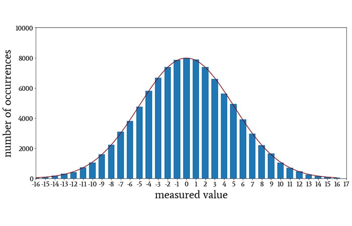
The Gaussian probability density function when we multiply P(x) by 100,000 and include the resulting curve in the histogram plot. 

     

Conclusion

I hope that you have enjoyed this article and that it has introduced the normal distribution with a good balance of practical and theoretical considerations. We’ll continue our discussion of the normal distribution in the next article.