How Standard Deviation Relates to Root-Mean-Square Values

If you're just joining in on this series about statistics in electrical engineering, you may want to start with the first article introducing statistical analysis and the second reviewing descriptive statistics. Most recently, we touched on sample-size compensation when calculating standard deviations—focusing specifically on Bessel’s correction.

In this article, we'll build on a previous article's discussion of standard deviation, which captures the averaged power of the random variations in a data set or digitized waveform. This averaged power is expressed as an amplitude, e.g., as volts instead of watts.

Electrical engineers deal with random variations all the time. We call them noise, and they ensure that no matter how good the weather is, we will have something to complain about.

We use the following formula to calculate standard deviation:

 

\[\sigma=\sqrt{\sigma^2}=\sqrt{\frac{1}{N-1}\sum_{k=0}^{N-1}(x[k]-\mu)^2}\]

 

Root Mean Square (RMS) Review

Most of us probably first learned about RMS values in the context of AC analysis. In AC systems, an RMS value of voltage or current is often more informative than a value that specifies the peak voltage or current, because RMS is a more direct path to power dissipation.

We can’t use a peak voltage or current value when calculating power dissipation because the voltage or current is constantly varying, and consequently the instantaneous power dissipation also varies. A calculation based on peak value would overestimate the time-averaged power.

RMS amplitudes allow us to calculate power dissipation as though we were working with DC quantities. More specifically, the RMS amplitude of a sinusoidal voltage or current is equal to the amplitude of a DC signal that would create the same amount of time-averaged power dissipation.

A 12 V battery connected to a 10 Ω resistor will generate 12²/10 = 14.4 W of (instantaneous and average) power. If we replace the battery with an AC supply voltage that has an RMS amplitude of 12 V, the (average) power will be the same.

Calculating RMS amplitudes is easy when we’re working with sinusoidal signals: we just divide the peak value by √2. The following diagram provides an interesting illustration of this relationship.

 

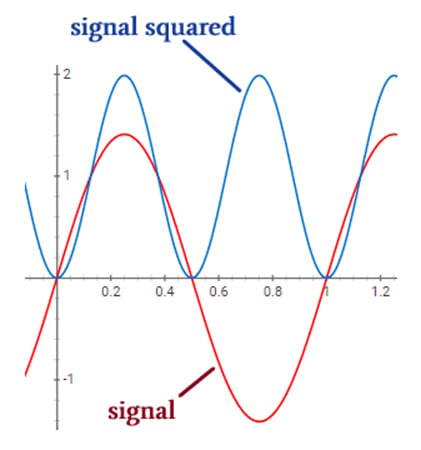
Here, we calculate the RMS amplitudes of sinusoidal signals by dividing the peak value by √2.

 

Power is proportional to the square of voltage or current. A DC voltage of 1 V connected to a circuit with resistance R will generate 1²/R = 1/R watts of power. We can see by inspection that the blue curve has an average value of 1; thus, since the blue curve is equal to the red curve squared, the average power generated by the red curve will also be 1/R.

Now notice the peak value of the red curve: it’s √2 (approximately 1.4). This confirms that we need to divide the peak value by √2 in order to identify the amplitude that will produce the correct average power when the standard formula—V²/R or I²R—is applied.

 

The Full RMS Calculation

Those of us who frequently work with AC electrical systems need to remember that RMS amplitudes are not limited to sinusoidal signals. Furthermore, the mathematical procedure that generates an RMS amplitude is significantly more complicated than dividing by √2.

It just so happens that with sinusoids, the procedure is equivalent to dividing by √2. This simplification does not apply to other types of signals such as square waves, triangular waves, or noise.

 

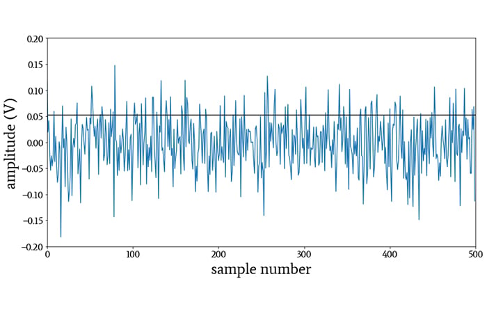
The horizontal line indicates the RMS amplitude of this noise waveform. The peak value of random noise tends to be 3 to 4 times higher than the RMS amplitude.

 

The actual RMS calculation—i.e., the calculation that we apply to signals in general—is expressed as follows:

 

\[X_{RMS}=\sqrt{\frac{1}{T_2-T_1}\int_{T1}^{T2}x(t)^2dt}\]

 

Here’s the procedure in words: Assume that x(t) is a time-domain signal that is periodic over the interval from time T₁ to time T₂. We square x(t), integrate this squared signal over the relevant interval, divide the integrated value by the length of the interval, and then take the square root.

Integrating from T₁ to T₂ and then dividing by (T₂–T₁) is analogous to summing all the values in the signal and dividing by the number of values. In other words, performing these two steps is the time-domain equivalent of calculating the arithmetic mean of a data set. Thus, we are taking the square root of the mean of the squared signal: root mean square.

 

RMS with Discrete Data

How would we convert the formula given above into something that we can apply to discrete data? In other words, how can we calculate the RMS amplitude of a digitized waveform?

Let’s look at it this way: First, we square individual values (e.g., x[1], x[2], x[3], etc.) instead of a function (e.g., x(t)). Next, when we move from a continuous-time signal to a discrete-time signal, integration becomes summation and a time interval becomes an “interval” of data points, i.e., the number of data points that were summed. Finally, we have the square root, which doesn’t change.

Thus, we can write our discrete-time RMS calculation as follows:

 

\[X_{RMS}=\sqrt{\frac{1}{N}(x[1]^2 + x[2]^2 + ... + x[N]^2)}\]

 

Is this beginning to look familiar? We’re squaring values, summing them, dividing by the number of values, and then taking the square root.

There are only two differences between this procedure and the procedure that we use to calculate standard deviation:

• With RMS, we divide by N; with standard deviation, we (usually) divide by N–1. We can ignore this difference because the use of N–1 is just an attempt to compensate for small sample size (see the previous article for more information).
• With RMS, we square the data points; with standard deviation, we square the difference between each data point and the mean.

If we’re trying to establish equivalency between RMS and standard deviation, the second difference might seem like a deal-breaker.

However, consider this: if the mean is zero, as is often the case in electrical signals, there is no difference between the RMS calculation and the standard-deviation calculation. In other words, for a signal with no DC offset, the standard deviation of the signal is also the RMS amplitude.

 

Conclusion

I’m not going to attempt to explore the full significance of this equivalency between standard deviation and root mean square. Nonetheless, before we finish up, I want to mention two interesting points that emerge from this discussion.

First, standard deviation gives us the “AC coupled” RMS amplitude of a waveform: we can calculate standard deviation when the DC offset of a signal is irrelevant, and this gives us the RMS amplitude of only the AC portion.

Second, standard deviation can be interpreted as a quantification of noise, and noise analysis is closely linked to the root mean square.