Sample-Size Compensation in Standard Deviation Calculations

This article continues our series on statistics for electrical engineers—the first of which introduced statistics as a means to analyze circuit behavior and characterize engineered systems. We then discussed specific methods—particularly in using the mean and median to find the central tendency of a dataset. 

Most recently, we touched on three descriptive statistical measures—average deviation, standard deviation, and variance in signal processing—to understand departures from those central tendencies. 

With our last article on standard deviation as a backdrop, we can now address another key aspect of the discussion: sample-size compensations in standard deviation calculations.

Divide by N or N–1?

If you’ve read the previous article, perhaps you noticed an apparent discrepancy in the formula that we use when we’re calculating the standard deviation of discrete data. The formula was given as follows:

\[\sigma=\sqrt{\sigma^2}=\sqrt{\frac{1}{N-1}\sum_{k=0}^{N-1}(x[k]-\mu)^2}\]

The standard deviation conveys the averaged power of the signal’s random deviations. However, when we calculate the average (i.e., the arithmetic mean) of something, we always divide by N (where N denotes the number of data points), not by N–1.

Why do we use N–1 when calculating the standard deviation?

Actually, we don’t always divide by N–1. We can calculate standard deviation using N instead of N–1, but in theory, the resulting number represents something different. I emphasize “in theory” because in the context of electrical engineering, the difference would often be insignificant. Nevertheless, it’s important to understand the underlying concept, which is rooted in the difference between a sample and a population.

Sample, Population, and Standard Deviation

Let’s say that you buy an op-amp (call it part number OPA100) and after some experimentation in the lab, you realize that the specs in the datasheet don’t give you enough information about input offset voltage at your application’s operating temperatures. To remedy this, you decide to buy 15 OPA100 op-amps (so N = 15), take some measurements, and generate some statistics based on this sample.

If the OPA100 has a typical offset voltage of 1 mV at the relevant operating temperature, the distribution of offset voltages in the 15-component sample might look something like this:

As you increase the sample size, the measured distribution will more closely resemble the normal distribution.

You’ve measured the offset voltage of each component and now you can calculate standard deviation, but first, you need to ask yourself a question: Do I want to calculate the standard deviation of the sample, or of the population? In other words, should I report the standard deviation of these 15 components in front of me, or should I attempt to report a standard deviation that applies to all OPA100 op-amps?

Standard Deviation of the Sample

If we’re working with a sample and we want to know the standard deviation of the sample, we divide by N. This makes sense—as mentioned above, we always divide by N when calculating the arithmetic mean, and the standard deviation involves the arithmetic mean of the power of the deviations in the data set.

So to continue our example, dividing by N would tell you the standard deviation of the 15 OPA100 op-amps that you purchased.

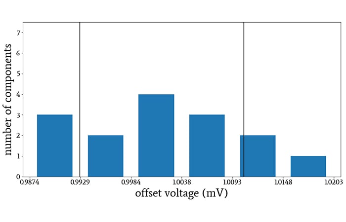
The vertical lines indicate the voltage values that are one standard deviation above and below the sample mean. I divided by N when calculating the standard deviation.

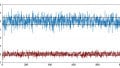
Another type of data set that electrical engineers frequently encounter is a digitized voltage signal, and as we saw in the previous article, standard deviation is a method of quantifying electrical noise.

If you want to know the standard deviation of the acquired signal, meaning the specific voltage levels that were digitized and stored in memory, you would divide by N when calculating the standard deviation. In this case, the acquired signal is the statistical sample.

Standard Deviation of the Population

If we’re working with a sample and we want to know the standard deviation of the population, we divide by N–1. “Population” refers to the entire group for which the obtained data points provide a representative sample. Using N–1 instead of N is a method of compensating for error associated with our finite sample size. The technique is called Bessel’s correction.

The correction is required because if we want to calculate the standard deviation of the population, we should use the population mean. But we usually don’t have access to the population mean. We have only the sample mean, which is an approximation of the population mean. It turns out that the standard deviation is consistently lower when we use the sample mean instead of the population mean, and dividing by N–1 instead of N mitigates this effect.

Thus, if you want to estimate the standard deviation of the offset voltage of all the OPA100 op-amps that have been manufactured, you should gather data from your 15-component sample and then divide by 14 instead of 15 when calculating the standard deviation.  

The vertical lines indicate the voltage values that are one standard deviation above and below the sample mean. I divided by N–1 when calculating the standard deviation.

Similarly, if you want to quantify the noise of a voltage signal based on a relatively short period of data acquisition, you would divide by N–1. In this case, the digitized data are the sample, and the signal itself is the population.

You can also think of this as follows: When we divide by N–1, we are focusing on the underlying processes that produce the noise in the analyzed signal, rather than measuring the effects of those processes within the slice of time represented by the acquired data points.

The Influence of Sample Size

Your engineer’s intuition probably tells you that Bessel’s correction is not the sort of thing that’s going to make or break your analysis, and in many cases this is true. In engineering applications, we often have an abundance of data, and we intuitively recognize that these large data sets will produce a sample mean that is, for all practical purposes, the same as the population mean. Thus, there’s no need to divide by N–1 instead of N.

However, we should keep in mind that this relationship is built into the correction. As N increases, the difference between N and N–1 becomes less significant with respect to the overall calculation. Thus, the use of N–1 applies desirable compensation when such compensation is needed (i.e., when sample size is small), and it has no noticeable effect when compensation is not needed (i.e., when sample size is large).

Conclusion

We’ve seen that standard deviation can be calculated in different ways depending on analytical intent and sample size. In the next article, we’ll explore the relationship between standard deviation and root-mean-square values.