Average Deviation, Standard Deviation, and Variance in Signal Processing

In the previous article on descriptive statistics for electrical engineers, we saw that both the mean and the median can convey the central tendency of a data set. Despite the fact that medians are less sensitive to outliers, means are used more frequently in electronics and digital signal processing. The arithmetic mean is, in fact, an essential statistical technique in electrical engineering.

However, we often need more than a mean to adequately describe or understand a data set.

When we report only the central tendency, we’re not considering an important aspect of the data—namely, the way in which values deviate from the central tendency.

 

Deviating from the Mean

Let’s imagine that we have digitized two analog input signals. If we convert the digital codes back into units of volts and plot the discrete-time waveforms, they look like this:

 

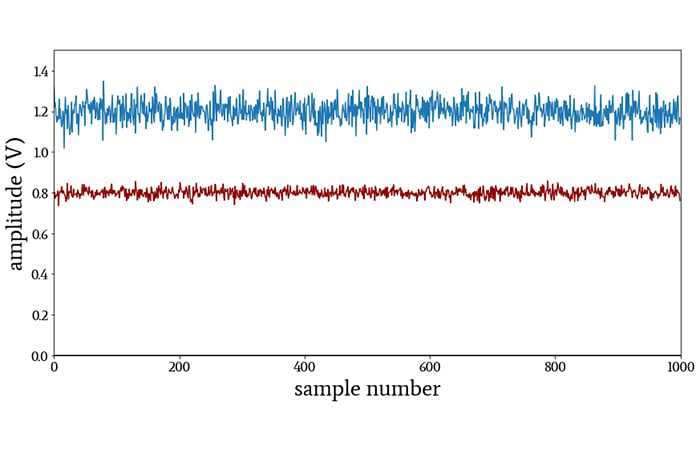
We can make a pretty good guess at the means just by looking at the plot: the central tendency of the blue signal is 1.2 V, and for the red signal it’s 0.8 V. But if we report nothing more than the means, we’ll give the impression that the only important difference between these two signals is the 0.4 V difference in the average value (or we might call it the DC level, or the DC offset). Clearly, there is more to the story.

An electrical engineer will instinctively identify these waveforms as steady DC signals (power-supply voltages, perhaps) that include quite a bit of noise.

More importantly, we immediately recognize that the blue signal is significantly noisier than the red signal. This major difference in noise performance is lost if we consider only the mean.

By the way, why do we perceive noise in these signals? Because

• the individual values visibly deviate from the average value,
• they do so in a way that appears random, and
• the deviations are small relative to the average value.

When a statistician sees small, random deviations from the mean, an electrical engineer sees noise.

 

Average Deviation

How noisy are these signals? Rather noisy? Very noisy? Let’s try to provide a more precise answer to that question. In other words, we need to quantify the deviation in these data sets.

My first instinct when quantifying deviation is to find the distance between each data point and the mean and then calculate the mean of all these distances. This would give you the average deviation (also called mean absolute deviation), i.e., the typical amount by which the values deviate from the central tendency. Here is the average deviation in mathematical language:

 

\[\text{average deviation}=\frac{1}{N}\sum_{k=0}^{N-1}|x[k]-\mu|\]

 

where N is the number of values in the data set, μ is the mean, and x[k] is the signal represented as a function of the discrete-time variable k.

 

In this plot, horizontal lines indicate the voltage levels that are one average deviation above and below the mean. 

 

Though average deviation is intuitive, it’s not the most common method of quantifying a signal’s tendency to deviate from the mean. For that, we need standard deviation.

 

Variance and Standard Deviation

In the context of electrical engineering, the problem with average deviation is that we’re averaging voltage (or current) differences, and therefore we’re operating in the domain of amplitude. The nature of noise phenomena is such that we emphasize power over amplitude when analyzing noise, and consequently we need a statistical technique that operates in the domain of power.

Fortunately, this is easily obtained. Power is proportional to the square of voltage or current, and consequently all we need to do is square the difference term before summation and averaging. This procedure results in a statistical measure called variance, denoted by σ² (pronounced as “sigma squared”):

 

\[\sigma^2=\frac{1}{N-1}\sum_{k=0}^{N-1}(x[k]-\mu)^2\]

 

We can describe variance as the averaged power of the signal’s random deviations expressed as power. This means that variance doesn’t have the same unit as the values that we started with. If we’re analyzing fluctuations in a voltage signal, variance has units of V² instead of V.

If we want to express a signal’s tendency to randomly deviate using the original unit, we must compensate for squaring each difference by applying the square root to the final value:

 

\[\sigma=\sqrt{\sigma^2}=\sqrt{\frac{1}{N-1}\sum_{k=0}^{N-1}(x[k]-\mu)^2}\]

 

This procedure generates a statistical measure known as standard deviation, i.e., the averaged power of the signal’s random deviations expressed as amplitude. Thus, if we’re analyzing a voltage signal, the standard deviation has units of V, despite the fact that we calculated the standard deviation using the square of the voltage deviations.

 

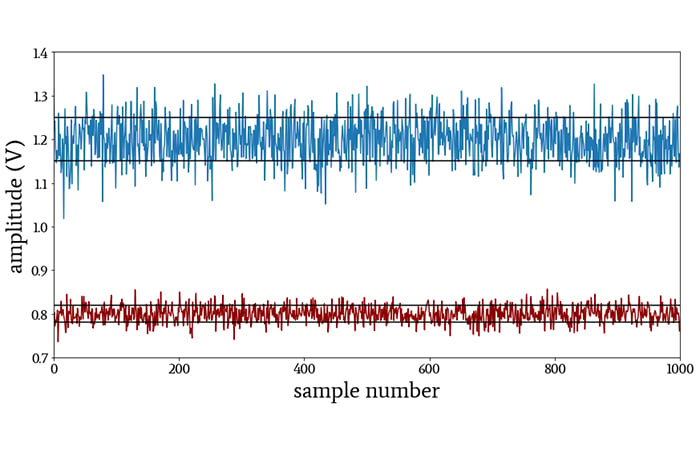
In this plot, horizontal lines indicate the voltage levels that are one standard deviation above and below the mean.

 

Variance and standard deviation express the same information in different ways. Though variance is, as I understand it, more convenient in certain analytical situations, standard deviation is usually preferred because it is a number that can be directly interpreted as a measure of a signal’s tendency to deviate from the mean.

 

Conclusion

Standard deviation and variance are essential statistical techniques that arise frequently in the sciences and the social sciences. I hope that this article has helped you to understand the basic connection between these concepts and electrical signals, and we’ll look at some interesting details related to standard deviation in the next article.