Facebook
 Google
 GitHub
 Linkedin
Basic Operations in Signal Processing: An Overview
Here we discuss some elementary operations that are important in signal processing and the practical scenarios for their applications.
Here we discuss some elementary operations that are important in signal processing and the practical scenarios for their applications.
Signals are used to represent any kind of fluctuation that occurs in our world. For example, when we speak, we produce sounds which can be represented as a function of few variables, or speech signals.
Signals can be represented either as analog or digital, depending on whether we represent it as a continuous function of time or only at definite time intervals, respectively.
Another example of signals can be found is in the communication field: radio, TV, or mobile.
There are electrocardiograms which represent the functioning of the heart in terms of waves.
It's easy to see that signals are woven into the threads of our day-to-day life whether we notice them or not.
Signal Manipulation
Since we can go through life with readily available signals, why do we need to complicate them by trying to ‘alter’ them?
You could argue that by trying to change them, we violate the natural human tendency of looking for convenience, whether technical or non-technical.
In order to answer this, let us move to the chemistry of our school days where we learned “the properties of elements differ from that of their compounds.”
This statement would also accompany an example of sodium chloride (NaCl), the common salt which is an essential nutrient for us. Sodium is a highly toxic, vigorously burning metal at room temperature, and chlorine is a poisonous greenish-yellow gas. Yet their combination results in the formation of crystalline salt which is in no way toxic.
A similar mode of explanation holds good in the case of signals as well. Suppose we have two elementary signals and then combine them by performing any kind of operation on them. We would get a new signal whose properties are different from those that make it up.
Now, if the properties of the signal obtained are better than those of the individual signals, then we would say that the complication brought about by our manipulation is worth doing.
Throughout this article, we cover ample of examples to emphasize (and re-emphasize) the fact conveyed by the above statement.
Types of Basic Operations
Now recall that any signal is represented as a function of variables that change its state. For example, if we have a progressive wave which changes with time, then we can represent in the form of y(t). Here t represents the independent variable while y is regarded as the dependent variable as its value depends on t.
As a result, when we say that we are ‘operating’ on a signal, we may either refer to the operations performed on the dependent or the independent variables. Depending on this, we can classify the basic operations performed over the signals into two types:
- Basic signal operations performed over the dependent variables
- Basic signal operations performed over the independent variables
In this article series, we will describe each of these types with adequate examples in each category and also discuss the practical scenarios in which they find their application.
I. Basic signal operations performed over the dependent variables
Here the manipulation of the signal will be accomplished by manipulating the dependent variable which represents the signal. For example, in the signal represented by x(t), we alter the variable ‘x’ and leave t as such.
1. Addition
The first and foremost operation which we will consider will be addition. The addition of signals is very similar to traditional mathematics. That is, if x1(t) and x2(t) are the two continuous time signals, then the addition of these two signals is expressed as x1(t) + x2(t).
The resultant signal can be represented as y(t) from which we can write
y(t) = x1(t) + x2(t)
Similarly for discrete time signals, x1[n] and x2[n], we can write
y[n] = x1[n] + x2[n]
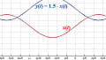
Figure 1 shows an example of addition operation performed over the continuous time signals x1(t) and x2(t).
Figure 1: Addition operation performed on two continuous time signals.
By following the green-coloured dotted line in Figure 1, you can note the value of y(t) at t = -1.5 to be 0 which is nothing but the summation of x1(t) at t = -1.5 which is 1 and that of x2(t) at t = -1.5 which is -1. Similarly, by moving along the purple-coloured dotted line, the value of y(-0.5) is seen to be 0 which is equal to x1(-0.5) + x2(-0.5) = -1 + 1.
Hence it can be concluded that all the values of the resultant signal y(t) can be obtained by adding the corresponding values of the signals x1(t) and x2(t). Although we have depicted the example of continuous time signals, the conclusion stated holds good even for discrete time signals.
Practical Scenario:
A practical aspect in which signal addition plays its role is in the case of transmission of a signal through a communication channel. This is because, here, we see that the undesired noise gets added up with the desired signal.
Another example which can be quoted is of dithering where the noise is added to the signal intentionally. This is because, when done so, one can effectively reduce undesired artifacts created as an aftermath of quantization errors.
2. Subtraction
Similar to the case of addition, subtraction deals with the subtraction of two or more signals in order to obtain a new signal. Mathematically it can be represented as
y(t) = x1(t) - x2(t) … for continuous time signals, x1(t) and x2(t)
and
y[n] = x1[n] - x2[n] … for discrete time signals, x1[n] and x2[n]
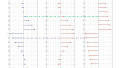
Subtraction operation performed over two discrete time signals x1[n] and x2[n] is shown in Figure 2.
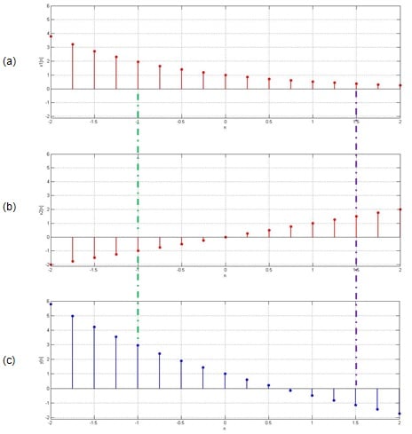
Figure 2: Subtraction operation performed on two discrete time signals.
Even in the case of subtraction operation, all the values of the resultant signal y[n] can be obtained by subtracting the corresponding values of the signals x1[n] and x2[n].
This is evident from the figure as the discontinuous green-colored dotted line shows y[-1] = 3 which is equal to x1[-1] - x2[-1] = 2 – (-1). Another example of a similar kind is shown by the discontinuous purple-colored dotted line, wherein y[1.5] = x1[1.5] - x2[1.5] = 0.4 – 1.5 = -1.1.
From the discussion presented, it can be stated that the conclusion we arrive at in the case of subtraction operation is very similar to that of the addition operation and applies to both continuous and discrete time signals.
Practical Scenario:
One practical aspect which connects with that of subtracting the signals is that of a Moving Target Indicator (MTI) used in radar communications (http://nptel.ac.in/courses/101108056/module3/lecture6.pdf). Here the most recent signal is subtracted from its previous version so as to obtain the signal which indicates just the moving targets by eliminating the stationary ones. This is very much necessary so as to facilitate PPI (Plan Position Indicator) display of radar systems.
Yet another example which extensively makes use of signal subtraction is the design of closed-loop control systems. Such systems employ negative feedback in order to accurately control an output variable, and this negative-feedback structure relies upon subtraction (the feedback signal is subtracted from the setpoint signal).
Summary
In this article, we presented an analysis on why signals are important and why we need to process them. We then categorized the basic signal operations based on whether they operate on dependent or independent variables.
Further, we discussed two operations viz., addition and subtraction which fall under the former type, by considering some practical usages for each of them.
The next article in this series will cover a few more basic signal operations along with a note on their applications.
Related Content