Facebook
 Google
 GitHub
 Linkedin
Basic Operations in Signal Processing: Multiplication, Differentiation, Integration
Here we discuss some elementary operations performed on the dependent variable representing the signal(s) and the examples in which they are applied.
Here we discuss some elementary operations performed on the dependent variable representing the signal(s) and the examples in which they are applied.
A Brief Review
In the first part of this article series, we saw that the signal operations can be classified into two types, viz.,
- Basic operations performed over the dependent variables
- Basic operations performed over the independent variables
In Part I, we discussed addition and subtraction operations which belong to the first category.
Now, in this article, we continue our analysis so as to know more regarding three more signal operations which belong to the same group (i.e., the basic operations which are performed over the dependent variables representing the signals).
1. Addition
Refer to the previous article.
2. Subtraction
Refer to the previous article.
3. Multiplication
The next basic signal operation performed over the dependent variable is multiplication. In this case, as you might have already guessed, two or more signals will be multiplied so as to obtain the new signal.
Mathematically, this can be given as:
y(t) = x1(t) × x2(t) … for continuous-time signals x1(t) and x2(t)
and
y[n] = x1[n] × x2[n] … for discrete-time signals x1[n] and x2[n]
Figure 1(c) shows the resultant discrete-time signal y[n] obtained by multiplying the two discrete-time signals x1[n] and x2[n] shown in Figures 1(a) and 1(b), respectively.
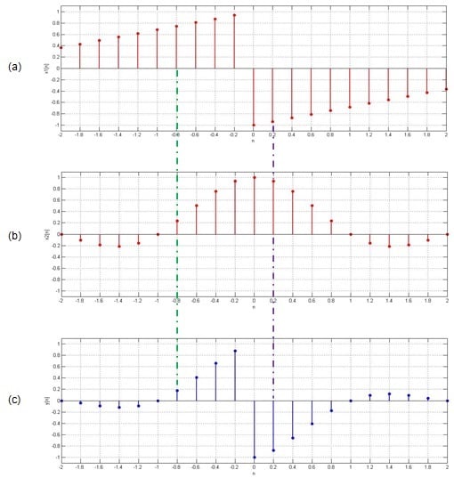
Figure 1. Multiplication operation performed over two discrete-time signals
Here the value of y[n] at n = -0.8 is seen to be 0.17, which is found to be equal to the product of the values of x1[n] and x2[n] at n = -0.8, which are 0.75 and 0.23, respectively. In other words, by tracing along the green dotted-dashed line, one gets 0.75 × 0.23 = 0.17.
Similarly, if we move along the purple dotted-dashed line (at n = 0.2) to collect the values of x1[n], x2[n], and y[n], we find that they are -0.94, 0.94, and -0.88, respectively. Here also we find that -0.94 × 0.94 = -0.88, which in turn implies x1[0.2] × x2[0.2] = y[0.2].
Thus, we can conclude that the multiplication operation results in the generation of a signal whose values can be obtained by multiplying the corresponding values of the original signals. This is true irrespective of whether we are dealing with a continuous-time or discrete-time signal.
Practical Scenario
Multiplication of signals is exploited in the field of analog communication when performing amplitude modulation (AM). In AM, the message signal is multiplied with the carrier signal so as to obtain a modulated signal.
Another example in which signal multiplication plays an important role is frequency shifting in RF (radio frequency) systems. Frequency shifting is a fundamental aspect of RF communication, and it is accomplished using a mixer, which is similar to an analog multiplier.
4. Differentiation
The next signal operation which is important in signal processing is differentiation. A signal is differentiated to determine the rate at which it changes. That is, if x(t) is the continuous-time signal, then its differentiation yields the output signal y(t), given by $$ y\left(t\right) = \frac{\text{d}}{\text{d}t}\left\{x\left(t\right)\right\} $$.
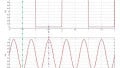
Figure 2 shows an example of a signal along with its differentiation. The figure shows the first derivative of a parabola—in Figure 2(a)—spanning from t = 0 to 2 to be a ramp—in Figure 2(b)—which has its values ranging from 0 to 4. The first derivative of the ramp in Figure 2(a) spanning from t = 2 to 6 is shown to be a constant amplitude of 1 in Figure 2(b).
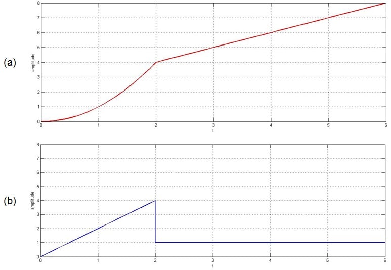
Figure 2. An original signal and its differentiation
Next, you should note that the differentiation operation is not restricted to continuous-time signals; it is also applicable to discrete-time signals.
Also, keep in mind that a signal can be differentiated more than once. For example, differentiating an original signal leads to a "first derivative" and differentiating this first derivative produces the "second derivative".
Practical Scenario
Differentiation of a signal takes the form of the gradient operator in the field of image or video processing. In the case of image processing, the gradient technique is a popular method which is used to detect the edges in the given image. With video processing, this operator is used for motion detection. This kind of processing is important in the field of robotics.
In addition, many control and tracking applications, such as in aeronautical systems, make use of real-time differentiators. This is because these applications require highly accurate data pertaining to velocity and acceleration. By using differentiators, this data can be obtained directly from position sensors, reducing the need for other sensors.
5. Integration
Integration is the counterpart of differentiation. If we integrate a signal x(t), the result y(t) is represented as $$ \int x\left(t\right) $$. Graphically, the act of integration computes the area under the curve of the original signal.
In Figure 3, a composite signal composed of a ramp extending from t = 0 to 2 and a constant value ranging from t = 2 to 5 is being integrated. The output obtained is shown in Figure 3(b); the integration of the ramp has resulted in a parabola (extending from t = 0 to 2), and the integration of the constant value has created a ramp (ranging from t = 2 to 5).
As with differentiation, we can integrate a signal multiple times.
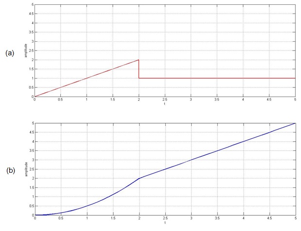
Figure 3. The integration operation
Practical Scenario
Integration is fundamental in signal-processing operations such as the Fourier transform, correlation, and convolution. These are, in turn, used to analyze different properties of a signal.
Other applications that employ integration are those in which small input currents are converted, via integration, into larger output voltages. Charge amplifiers are used with piezoelectric sensors, photodiodes, and CCD imagers. Also, charge amplifiers can be used to convert an accelerometer output into velocity and displacement signals, because integrating acceleration yields velocity, and integrating velocity yields displacement.
Summary
This article discusses three operations that act on a signal's dependent variable: multiplication, differentiation, and integration.
In the next article of this series, we will discuss the second category of basic signal operations, i.e., those which manipulate the characteristics of a signal by influencing its independent variable.