Facebook
 Google
 GitHub
 Linkedin
Basic Signal Operations in DSP: Constant-Valued and Alternating Signals
In this article, we’ll discuss a few elementary signal operations by considering one of the signals to be constant-valued.
In this article, we’ll discuss a few elementary signal operations by considering one of the signals to be constant-valued.
Signals can mathematically represent variations in parameters.
If there is a consistent change in the value of a signal with respect to time, then we get an alternating signal. On the other hand, if the value of the signal remains constant for a very wide range, then we get a constant-valued signal. These concepts are illustrated by alternating current (AC) and direct current (DC), respectively.
The field of signal processing has many examples of signal manipulating operations. You can see some of the basic operations in the first articles of this series:
- Basic Operations in Signal Processing: An Overview
- Basic Operations in Signal Processing: Multiplication, Differentiation, Integration
Our example signals in these articles continuously varied over time. Essentially, we didn’t deal with constant-valued signals.
In this article, however, we’ll review the same basic signal operations as before but we will use constant-valued signals as our examples.
Addition/Subtraction of an Alternating Signal with a Constant-Valued Signal
Adding Signals: Positive Clamping
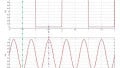
Let’s start with a sinusoidal signal as shown by the red curve in Figure 1.
Now, let’s add a constant-valued signal of amplitude 1.5 to it. Our output signal becomes y(t) = x(t) + 1.5. The plot obtained is shown by the blue curve in the same figure.
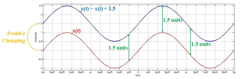
Figure 1. Addition of an alternating signal with a constant-valued signal of amplitude 1.5
As you can see, y(t) is the same as x(t) but shifted all along its trace by a magnitude of 1.5 (the constant-value added to it).
This is a good demonstration of what happens when we add a constant-valued signal to an alternating signal—the latter is shifted to the level of the former. This shift in the reference level of the alternating signal is termed “clamping”. Since, in this example, there’s a shift towards a positive value, we can call it “positive clamping”.
What happens if we add the alternating signal the constant-valued signal instead? That mathematical equation would be y(t) = 1.5 + x(t).
However, the result would be the same. Why? As in simple math, addition is commutative which means that x(t) + 1.5 = 1.5 + x(t).
Subtracting Signals: Negative Clamping
Next, let’s try subtracting. We’ll start by subtracting our example constant-valued signal from our alternating signal. Let y(t) be x(t) - 1.5.
The output corresponding to this is shown as the blue curve in Figure 2. By comparing this curve with the red curve representing the original signal, we can see that the amplitude of the signal has been reduced by 1.5 overall.
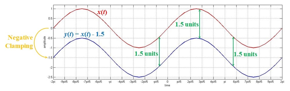
Figure 2. Effect of subtracting a constant-valued signal of amplitude 1.5 from an alternating signal
A direct consequence of this, as evident from the figure, is the clamping of the alternating signal to -1.5. Since the clamping is towards a negative value, we call it “negative clamping”.
When we write this out as y(t) = x(t) - 1.5 as y(t) = - 1.5 + x(t), we can see that, even in this case, clamping must occur but towards a negative value.
As a continuation, let us now try to reverse the order of subtraction. That is, let our output signal be y(t) = 1.5 - x(t) instead of y(t) = x(t) - 1.5.
Figure 3 shows the result corresponding to this operation:
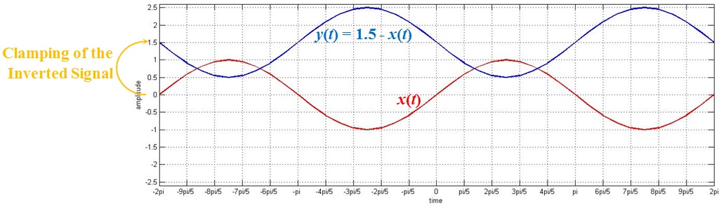
Figure 3. Effect of subtracting an alternating signal from a constant-valued signal of amplitude 1.5
At first glance, it appears that this throws our idea of “clamping” out the window. However, that’s not completely true.
Why?
Observe closely. The blue curve in the figure is the alternating signal but inverted along the horizontal axis and clamped at the level 1.5.
Our equation for the output in this case is y(t) = 1.5 - x(t) which the same thing as y(t) = 1.5 + {-x(t)}. This indicates that, here, the inverted x(t) should get clamped to a level of 1.5.
Conclusions about Adding or Subtracting
We can conclude that the addition or subtraction of a constant-valued signal with that of an alternating one invariably results in clamping of the alternating signal to a value decided by the constant.
Electronically speaking, the circuits which give rise to clamping are called “clampers”.
So we know that that addition/subtraction operations performed amongst signals where at least one of them is constant-valued find their use in all scenarios in which clampers are applied. Base-line stabilizers, DC restoration circuits, and the circuits used to establish compatibility between the operating range of the device with that of the incoming signal are only a few examples of applications you might see these operations in action.
Effect of Multiplying a Constant-Valued Signal with an Alternating Signal
In this section, we’ll look at the effects of multiplying a constant-valued signal by an alternating one. In particular, let’s multiply a constant-valued signal of amplitude 1.5 with an alternating signal, x(t), which is a sine wave of period 2π (shown as a red curve in Figure 4).
The resultant plot is shown as a blue curve in Figure 4:
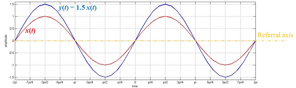
Figure 4. Multiplication of a constant-valued signal with amplitude 1.5 by an alternating signal
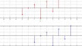
From the graph, you can see that the value of x(t) at –π/2 is -1 while that of y(t) is -1.5 (that is, 1.5 times the value of x(t)). Similarly, at the time instants 0, π/2, and 3π/2, we have the values of y(t) as 0, 1.5, and -1.5 respectively. You’ll note that these are the values of x(t) (0, 1, and -1, respectively) multiplied by 1.5.
This indicates that, when we multiply a signal by a constant-value, we get a signal which has its values multiplied by the same factor.
At this point, we should discuss an important point with respect to Figure 4. Unlike with addition and subtraction (like in Figures 1 through 3), the multiplication operation does not result in clamping of the signal. As with addition, however, multiplication is commutative, giving us y(t) = 1.5 x(t) = x(t) 1.5.
Conclusions about Multiplying
From the discussion presented, it is clear that multiplication of a signal with a constant greater than one increases its amplitude without clamping it. This is essentially the amplification of the input signal by a factor as decided by the value of constant. Hence, this kind of multiplication operation finds its use in all the cases wherein electronic amplifiers find their use.
A few example applications of this are low-noise amplifiers in communication systems, audio/video amplifiers of radio/television sets, and operational amplifiers which form an integral part of numerous electronic circuits.
Differentiation and Integration of a Constant-Valued Signal
As per mathematics, differentiation of a constant would be zero. The same is true even in the case of signals. That is to say, by differentiating a constant-valued signal, we would get a zero-valued signal. This is the operational principle behind the working of DC blocking capacitors used in many electronic designs.
On the other hand, if we integrate a constant-valued signal, we get a ramp whose slope is decided by the value of the constant. Circuits like constant-current ramp generators work on this principle.
Summary
In this article, we analyzed the results produced when we subject constant-valued signals to basic signal operations. We also saw how operations like addition/subtraction, multiplication, differentiation, and integration result in effects like clamping, amplification, DC blocking and ramp generation, respectively.