 Facebook
 Google
 GitHub
 Linkedin
Basic Signal Operations in DSP: Time Shifting, Time Scaling, and Time Reversal
This article presents a look at the basic signal operations performed over the independent variable(s) affecting the signal and the scenarios in which they find their application.
This article presents a look at the basic signal operations performed over the independent variable(s) affecting the signal and the scenarios in which they find their application.
A Brief Review
In the first part of this article series, Basic Operations in Signal Processing: An Overview, we categorized the basic signal operations into two types depending on whether they operated on dependent or independent variable(s) representing the signals.
Addition, subtraction, multiplication, differentiation, and integration fall under the category of basic signal operations acting on the dependent variable. Brief notes on each of them along with their practical applications were discussed in both the overview article linked above and in part two of this series, Basic Operations in Signal Processing: Multiplication, Differentiation, Integration.
Now, in this article, we concentrate on the basic signal operations which manipulate the signal characteristics by acting on the independent variable(s) which are used to represent them. This means that instead of performing operations like addition, subtraction, and multiplication between signals, we will perform them on the independent variable. In our case, this variable is time (t).
1. Time Shifting
Suppose that we have a signal x(t) and we define a new signal by adding/subtracting a finite time value to/from it. We now have a new signal, y(t). The mathematical expression for this would be x(t ± t0).
Graphically, this kind of signal operation results in a positive or negative “shift” of the signal along its time axis. However, note that while doing so, none of its characteristics are altered. This means that the time-shifting operation results in the change of just the positioning of the signal without affecting its amplitude or span.
Let's consider the examples of the signals in the following figures in order to gain better insight into the above information.
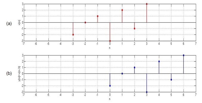
Figure 1. Original signal and its time-delayed version
Here the original signal, x[n], spans from n = -3 to n = 3 and has the values -2, 0, 1, -3, 2, -1, and 3, as shown in Figure 1(a).
Time-Delayed Signals
Suppose that we want to move this signal right by three units (i.e., we want a new signal whose amplitudes are the same but are shifted right three times).
This means that we desire our output signal y[n] to span from n = 0to n = 6. Such a signal is shown as Figure 1(b) and can be mathematically written as y[n] = x[n-3].
This kind of signal is referred to as time-delayed because we have made the signal arrive three units late.
Time-Advanced Signals
On the other hand, let's say that we want the same signal to arrive early. Consider a case where we want our output signal to be advanced by, say, two units. This objective can be accomplished by shifting the signal to the left by two time units, i.e., y[n] = x[n+2].
The corresponding input and output signals are shown in Figure 2(a) and 2(b), respectively. Our output signal has the same values as the original signal but spans from n = -5 to n = 1 instead of n = -3 to n = 3. The signal shown in Figure 2(b) is aptly referred to as a time-advanced signal.
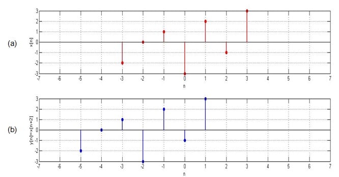
Figure 2. Original signal and its time-advanced version
For both of the above examples, note that the time-shifting operation performed over the signals affects not the amplitudes themselves but rather the amplitudes with respect to the time axis. We have used discrete-time signals in these examples, but the same applies to continuous-time signals.
Practical Applications
Time-shifting is an important operation that is used in many signal-processing applications. For example, a time-delayed version of the signal is used when performing autocorrelation. (You can learn more about autocorrelation in my previous article, Understanding Correlation.)
Another field that involves the concept of time delay is artificial intelligence, such as in systems that use Time Delay Neural Networks.
2. Time Scaling
Now that we understand more about performing addition and subtraction on the independent variable representing the signal, we'll move on to multiplication.
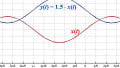
For this, let's consider our input signal to be a continuous-time signal x(t) as shown by the red curve in Figure 3.
Now suppose that we multiply the independent variable (t) by a number greater than one. That is, let's make t in the signal into, say, 2t. The resultant signal will be the one shown by the blue curve in Figure 3.
From the figure, it's clear that the time-scaled signal is contracted with respect to the original one. For example, we can see that the value of the original signal present at t = -3 is present at t = -1.5 and those at t = -2 and at t = -1 are found at t = -1 and at t = -0.5 (shown by green dotted-line curved arrows in the figure).
This means that, if we multiply the time variable by a factor of 2, then we will get our output signal contracted by a factor of 2 along the time axis. Thus, it can be concluded that the multiplication of the signal by a factor of n leads to the compression of the signal by an equivalent factor.
Now, does this mean that dividing the variable t by a number greater than 1 will cause the signal to become expanded? That is, if we divide the variable t by a factor of n, will we get a signal which is stretched by an equivalent factor?
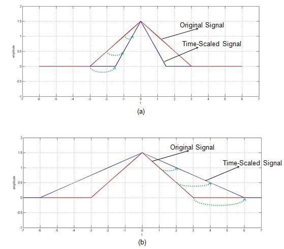
Figure 3. Original signal with its time-scaled versions
Let's check it out.
For this, let's consider our signal to be the same as the one in Figure 3 (the red curve in the figure). Now let's multiply its time-variable t by ½ instead of 2. The resultant signal is shown by the blue curve in Figure 3(b). You can see that, in this time-scaled signal indicated by the green dotted-line arrows in Figure 3(b), we have the values of the original signal present at the time instants t = 1, 2, and 3 to be found at t = 2, 4, and 6.
This means that our time-scaled signal is a stretched-by-a-factor-of-n version of the original signal. So the answer to the question posed above is "yes."
Although we have analyzed the time-scaling operation with respect to a continuous-time signal, this information applies to discrete-time signals as well. However, in the case of discrete-time signals, time-scaling operations are manifested in the form of decimation and interpolation.
Practical Applications
Basically, when we perform time scaling, we change the rate at which the signal is sampled. Changing the sampling rate of a signal is employed in the field of speech processing. A particular example of this would be a time-scaling-algorithm-based system developed to read text to the visually impaired.
Next, the technique of interpolation is used in Geodesic applications (PDF). This is because, in most of these applications, one will be required to find out or predict an unknown parameter from a limited amount of available data.
3. Time Reversal
Until now, we have assumed our independent variable representing the signal to be positive. Why should this be the case? Can't it be negative?
It can be negative. In fact, one can make it negative just by multiplying it by -1. This causes the original signal to flip along its y-axis. That is, it results in the reflection of the signal along its vertical axis of reference. As a result, the operation is aptly known as the time reversal or time reflection of the signal.
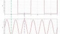
For example, let's consider our input signal to be x[n], shown in Figure 4(a). The effect of substituting –n in the place of n results in the signal y[n] as shown in Figure 4(b).
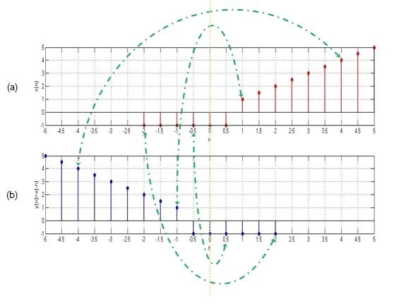
Figure 4. A signal with its reflection
Here you can observe that the value of x[n] at the time instant n = -2 is -1. This is equal to the value of y[n] at n = 2. Likewise, x[-0.5] = y[0.5] = -1, x[1] = y[-1] = 1, and x[4] = y[-4] = 4 (as indicated by the green dotted-dashed-line arrows).
This indicates that the graph of y[n] is nothing but the original signal x[n] reflected along the vertical axis (shown as a dotted orange line in the figure).
This applies to both continuous- and discrete-time signals.
Practical Applications
Time reversal is an important preliminary step when computing the convolution of signals: one signal is kept in its original state while the other is mirror-imaged and slid along the former signal to obtain the result. Time-reversal operations, therefore, are useful in various image-processing procedures, such as edge detection.
A time-reversal technique in the form of the time reverse numerical simulation (TRNS) method can be effectively used to determine defects. For example, the TRNS method aids in finding out the exact position of a notch which is a part of the structure along which a guided wave propagates.
Conclusion
This article presents an analysis of the following signal operations: time shifting, time scaling, and time reversal. In addition, we briefly went over practical applications for these operations.
Related Content


Great work!