The Statistical Nature of Noise Analysis: An Introduction

This article is an intuitive introduction to the statistical nature of noise and the basic calculations required to combine noise sources in a circuit.

There are different ways to consider noise in electrical circuits. The noise considered here is unwanted signal originating within circuit components. For example, Johnson noise from resistors or input noise voltage of op-amps.

This discussion assumes the noise sources have two characteristics:

• First, multiple sources are uncorrelated.
• Second, the probability of a particular amplitude at a point in time follows a Gaussian or normal distribution which is the case for many sources.

We'll take a look at how to represent noise with data sets, the RMS amplitude of noise sources (and how to convert that information to peak-to-peak amplitude), and discuss an example of noise analysis in a circuit.

 

Sample Data Set with a Normal Distribution

I downloaded a set of random numbers from a random number website. These are true random numbers derived from a physical process and not pseudo-random numbers. There are 10,000 samples with a Gaussian or normal distribution and standard deviation of 10. The mean or center of the distribution is 0. Here are the first five and last five numbers in the series, so that you can get a sense of the range of values.

 

Table 1. First 5 and last 5 values in a random sample of process data with mean 0 and standard deviation 10.

Sample	Value
1	-17.6
2	-9.63
3	8.26
4	8.44
5	-6.65
9,996	14.1
9,997	-16.3
9,998	-15.2
9,999	-0.30
10,000	15.88

 

For our purposes, it is useful to think of the data as a series of samples in time as if viewing noise with an oscilloscope. In other words, treating the data as noise in the time domain. FIgure 1 displays the first 500 samples. It looks like noise to me!

 

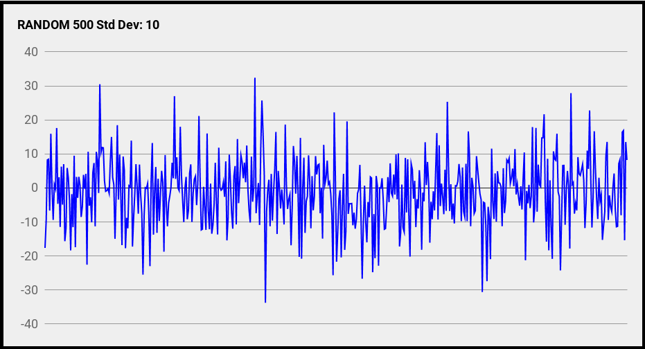
Figure 1. First 100 values in a random sample of process data with mean 0 and standard deviation 10. Data courtesy of Random.org

 

In Figure 2, all 10,000 samples are shown as a histogram. This is the classic normal distribution or “bell” curve. I have drawn a line in the center at 0 for the mean and a line to the left at -10 to identify one standard deviation.

 

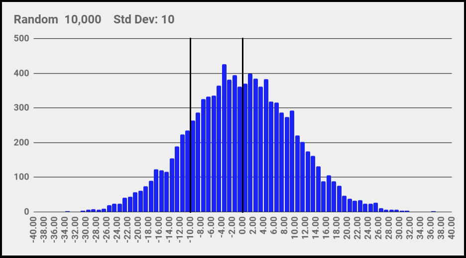
Figure 2. Histogram of a random sample of process data with mean 0 and standard deviation 10. Data courtesy of Random.org

 

Noise Sources and the Normal Distribution

How does this data set relate to electronic noise? 

If a noise source has a normal distribution, the RMS amplitude of the source is the same as the standard deviation of the distribution. In the plot of the first 500 samples, the RMS amplitude is the standard deviation of 10. A plot of all 10,000 samples (see below) will also have an RMS amplitude of 10.

The other important relationship is with the amplitude extremes in the data. The largest samples occur much less frequently than amplitudes near 0. There is a lot more about these “outliers” later in the article.

If you'd like to learn more about visualizing noise sources, you can also learn more about how to simulate noise sources in LTspice here. 

 

Adding Noise Sources

Since noise sources are uncorrelated, the amplitudes do not add arithmetically. In other words, for two noise sources, $$V_{T}≠V_{A}+V_{B}$$. They are added as the square root of the sum-of-their-squares; this is often referred to as RSS (root sum square) summation. For example, the sum of three noise sources is

 

$$V_{T} = \sqrt{(V_{A})^2 + (V_{B})^2 + (V_{C})^2}$$

 

To see this intuitively, three groups of 500 continuous samples were taken from the data set to form three, 1 x 500 matrices (vectors). Vector A is sampled 1 to 500, B is 501 to 1000, and C is 1001 to 1500. Even though the groups are from the same data set, they are uncorrelated. Then, add the three vectors.

 

D = A + B + C

 

This is how three sources add in a circuit over time. Figure 3 is a plot of D.

 

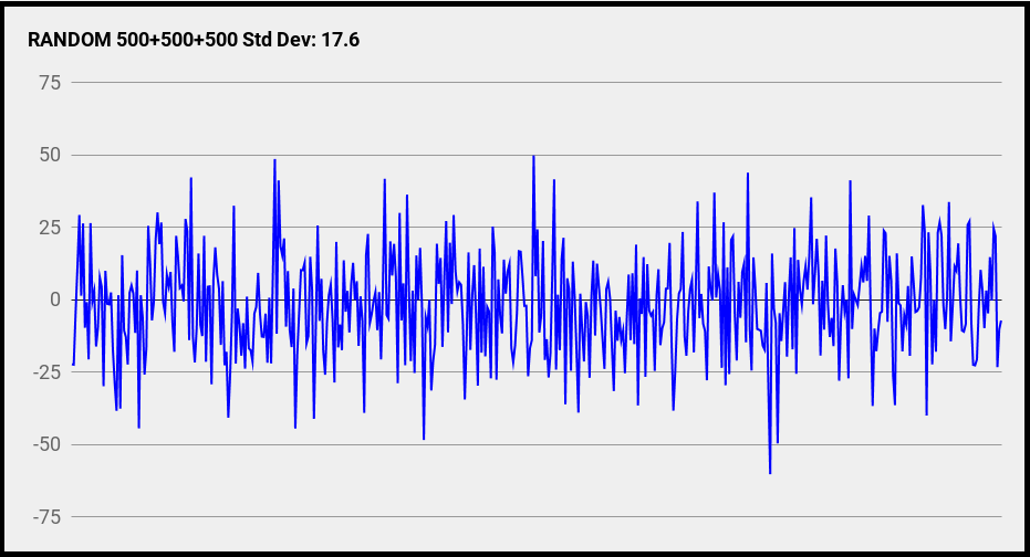
Figure 3. The result of adding three sets of uncorrelated random data.

 

In the plot of D, almost all the samples are within +/-50. The standard deviation of the 500 samples in D is 17.6.

Now, let’s calculate the sum of the RMS amplitude of the three sources.

 

$$V_{T} = \sqrt{(V_{A})^2 + (V_{B})^2 + (V_{C})^2}$$

$$V_{T} = \sqrt{10^2 + 10^2 + 10^2}$$

$$V_{T} = \sqrt{300}$$

$$V_{T} = 17.3$$

 

We have calculated the sum of the three sources in two different ways. One calculates the sum as three sources with RMS amplitude using the RSS method. The other adds the data point by point and determines the standard deviation of the result.

$$17.3 ≅ 17.6$$

Pretty close! RMS amplitudes and the RSS method are useful, but they are not particularly intuitive. The vector example, on the other hand, is somewhat intuitive. We can imagine uncorrelated sources varying in time and adding in a circuit.

 

Adding Two Equal Noise Sources

If two noise sources are the same amplitude $$V_{A} = V_{B}$$, the total noise is

 

$$V_{T} = \sqrt{(V_{A})^2 + (V_{B})^2}$$

$$V_{T} = \sqrt{2\times (V_{A})^2}$$

$$V_{T} = \sqrt{2}\times V_{A}$$

$$V_{T} = 1.414\times V_{A}$$

 

This is a useful relationship to memorize. For example, this equation gives the total noise for two JFETs at the input of a differential amplifier.

Conversely, if the total noise is known, the amplitude of one of the sources is

 

$$V_{T} = \sqrt{2}\times V_{A}$$

$$V_{A}=\frac{V_{T}}{\sqrt{2}}$$

$$V_{A} = 0.707\times V_{T}$$

 

Adding a Small Noise Source to a Large Noise Source

If one noise source is much larger than another source, the smaller source can often be ignored. For example, if one source is 10 times larger than the other,

 

$$V_{T} = \sqrt{(10\times V)^2 + V^2}$$

$$V_{T} = \sqrt{100\times V^2 + V^2}$$

$$V_{T} = \sqrt{101\times V^2}$$

$$V_{T} ≈ 10.05\times V$$

 

The smaller noise source only adds 0.5% to the total noise! This is negligible in the noise world, or as the saying goes, “It’s in the noise”.

This relationship explains why noise in a preamp is important but noise in later stages is often not so important—the preamp noise experiences high amplification, but the noise generated by later stages does not. It is also useful when we want to simplify estimates of noise in a circuit. Just throw out the small sources.

 

Converting RMS Amplitude to Peak-to-Peak Amplitude

When we’re working with noise, converting RMS amplitude to peak-to-peak is a bit tricky. The conversion must be considered statistically, and in contrast to conversion involving sine waves, it does not employ a precise value. Figure 4 is a plot of all 10,000 samples in the data set.

 

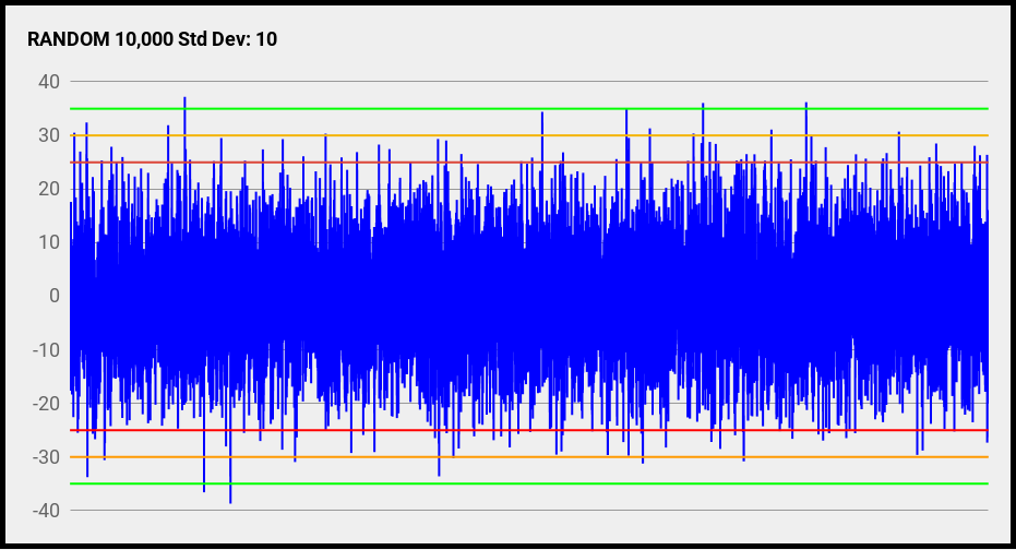
Figure 4. 10,000 random sample of process data with mean 0 and standard deviation 10. Data courtesy of Random.org

 

Notice the extreme positive and negative peaks. There are not very many of them. Furthermore, it is the nature of a normal distribution that there are no guaranteed maximum and minimum values. In theory, if we wait long enough, a larger peak will come along.

So, an assumption must be made of where to “draw the line” representing a definition of peak-to-peak. I added three sets of peak-to-peak lines to the plot in Figure 4. They are placed at multiples of the standard deviation, as shown in Table 2.

 

Table 2. Three sets of calculations for peak-to-peak and range as multiples of the RMS (standard deviation) for the noise.

Line Pair	x RMS	Peak-to-Peak Value	Range
Red	5	50	+/-25
Orange	6	60	+/-30
Green	7	70	+/-35

 

To me, the multiplication factor is application dependent. Selecting a peak-to-peak factor may be important to prevent clipping in an amplifier or to not exceed a trigger threshold. A fire alarm may need a very large factor to prevent false alarms!

Another way to view RMS to peak-to-peak uses the normal distribution. Figure 5 is the graph with red lines at 5 times the RMS value (+/-25 = 50).

 

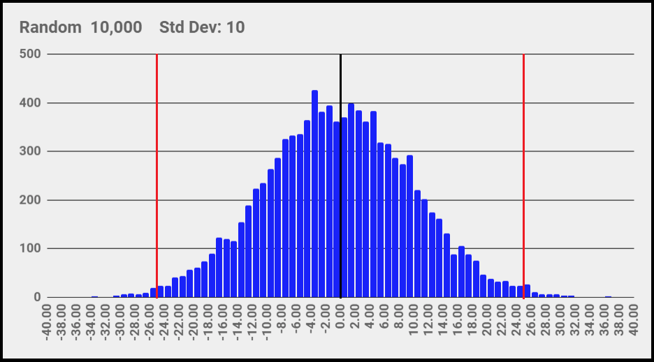
Figure 5. Red lines indicate peak-to-peak values 5 times the RMS value (50 = 5 x 10).

 

The percentage of samples outside the peak-to-peak “window” is calculated statistically. Thankfully, there are charts and online calculators. The topic is “cumulative distributions,” and it can be tricky finding the right online calculator. Table 3 has the percentage of points outside the window or, in other words, the amount of time the noise is outside the window.

 

Table 3. Relationship between the peak-to-peak multiples of the RMS and the percentage of outliers that exceed these values.

Line Pair	x RMS	% Out
Red	5	1.2%
Orange	6	0.27%
Green	7	0.046%

 

6 x RMS is used a lot. Some people like 6.6 because it corresponds to 0.10%. Nice number but, in my opinion, no more meaningful than others without considering the application. I like 6.283185 (≅2π). I’m claiming it!

Remember, the data is random and is described with probabilities. It is impossible to know when a noise source will go outside the window. Even if the window is large, going outside the window could happen in the next second or not for a week or not at all.

 

Circuit Example

This section uses the concepts above to analyze a preamp and determine the total output noise. I use a “spot noise” calculation for noise at 1 kHz and a bandwidth of 1 Hz.

The purpose here is to test combining multiple noise sources. The manual calculations are compared to a noise simulation done with LTspice, which is a popular and free circuit simulator from Analog Devices. If you'd like to learn more about this process, you should also consider checking out our tutorial on noise analysis in LTspice by Steve Colley. The circuit shown in Figure 6 is a non-inverting amplifier—using an ADA4627 op-amp from Analog Devices—with an input signal source represented by V3. A source resistance of 100Ω is in series with the input. This simulates a platinum RTD sensor.

 

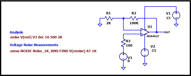
Figure 6. Circuit schematic of a non-inverting amplifier for noise simulation.

 

All the noise sources are listed in the Table 4.

Table 4. Details of the noise sources for the non-inverting amplifier

Source	Source (V/√Hz @1kHz)	Gain	Output (V/√Hz @1kHz)	Description
R1	5.75E-9	50	287.5E-9	Johnson noise
R2	40.7E-9	1	40.7E-9	Johnson noise
R3	1.3E-9	51	65.6E-9	Johnson noise
U1:VN	5.04E-9	51	257.0E-9	Input voltage noise
U1:IN+	0.22E-12	51	0.01E-9	+Input current noise through R3
U1:IN-	4.5E-12	50	0.22E-9	-Input current noise through R1

 

R1, R2, and R3 are Johnson noise sources at 27℃. The op-amp input voltage noise and input current noise are found by running special LTspice simulations and checking the datasheet specifications.

The input current noise is a source at each op-amp input (+ and -). The input current noise from the - input is multiplied by R1 to produce an input voltage noise, and the input current noise from the + input is multiplied by R3.

Finally, the noise at the output for each source is calculated by multiplying each source by its gain. All voltages are RMS. None of that peak-to-peak stuff here!

The individual output noise sources are combined using RSS addition to produce the total output noise.

 

$$V_{T} = \sqrt{287.5nV^2+40.7nV^2+65.6nV^2+257nV^2+0.01nV^2+0.22nV^2}$$

$$V_{T} = 393.3\frac{nV}{\sqrt{Hz}}$$

 

Running a noise simulation in LTspice produces a simulated total output noise of $$393.4\frac{nV}{\sqrt{Hz}}$$. Not bad! 

The effect of adding a small source to a large one is tested by comparing the output noise from only the two largest sources, R1 and U1: V_N, to the output noise with all the sources.

 

$$V_{T} = \sqrt{287.5nV^2 + 257nV^2}$$

$$V_{T} = 385 \frac{nV}{\sqrt{Hz}}$$

 

The result is only 2% lower! In my experience, there are often noise sources to ignore in a quick estimate. Obvious ones here are the op-amp input current noise since the source resistances are small and the noise currents flowing through these resistors are very small.

A comment about noise simulation. When learning, it is best to go through a few calculations by hand. However, this is tedious and error-prone. Switching to a simulator such as LTspice is a big help, especially when noise bandwidth is included.

The analysis here is relatively simple because it is a spot noise calculation. Please check out our resources below for more information!

More Information on Noise

• Basic Circuit Simulation with LTspice
• Intermediate LTspice Tutorial
• Noise Analysis Using LTspice Tutorial
• What Is Electrical Noise and Where Does It Come From?
• Using LTSpice for Amplifier Noise Measurement