Facebook
 Google
 GitHub
 Linkedin
Understanding Parametric Tests, Skewness, and Kurtosis
This article introduces important subcategories of inferential statistical tests and discusses descriptive statistical measures related to the normal distribution.
Welcome to our series on statistics in electrical engineering. So far, we've reviewed statistic analysis and descriptive analysis in electrical engineering, followed by a discussion of average deviation, standard deviation, and variance in signal processing.
Next, we reviewed sample-size compensation in standard deviation calculations and how standard deviation related to root-mean-square values.
Now, we've moved on to an exploration of normal distribution in electrical engineering—specifically, how to understand histograms, probability, and the cumulative distribution function in normally distributed data. This article extends that discussion, touching on parametric tests, skewness, and kurtosis.
When the Normal Distribution Doesn't Look Normal
In previous articles, we explored the normal (aka Gaussian) distribution both as an idealized mathematical distribution and as a histogram derived from empirical data. If a measured phenomenon is characterized by a normal distribution of values, the shape of the histogram will be increasingly consistent with the Gaussian curve as sample size increases.
This leads us to an interesting question, though: How do we know if a phenomenon is characterized by a normal distribution of values?
If we have a large quantity of data, we can simply look at the histogram and compare it to the Gaussian curve. With smaller data sets, however, the situation is more complicated. Even if we are analyzing an underlying process that does indeed produce normally distributed data, the histograms generated from smaller data sets may leave room for doubt.
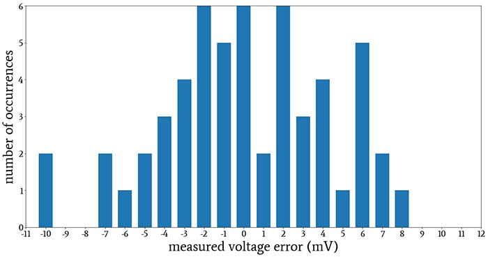
Are these data normally distributed?
In this article, we’ll discuss two descriptive statistical measures—called skewness and kurtosis—that help us to decide if our data conform to the normal distribution.
First, though, I want to examine a related question: Why do we care whether or not a data set conforms to the normal distribution?
Parametric vs. Nonparametric Tests
There are various statistical methods that help us analyze and interpret data and some of these methods are categorized as inferential statistics. We often use the word “test” when referring to an inferential statistical procedure and these tests can be either parametric or nonparametric.
The distinction between parametric and nonparametric tests lies in the nature of the data to which a test is applied. When a data set exhibits a distribution that is sufficiently consistent with the normal distribution, parametric tests can be used. When the data are not normally distributed, we turn to nonparametric tests.
Examples of parametric tests are the paired t-test, the one-way analysis of variance (ANOVA), and the Pearson coefficient of correlation. The nonparametric alternatives to these tests are, respectively, the Wilcoxon signed-rank test, the Kruskal–Wallis test, and Spearman’s rank correlation.
Why “Parametric” and “Nonparametric”?
If you’re feeling confused about this parametric/nonparametric terminology, here’s an explanation: A parameter is a characteristic of an entire population—for example, the mean height of all Canadians, or the standard deviation of output voltages generated by all the REF100 reference-voltage ICs that have been manufactured (I made up that part number).
We usually can’t know a parameter with certainty, because our data represent only a sample of the population. We can, however, produce an estimate of a parameter by computing the corresponding statistical value based on the sample.
Parametric tests rely on assumptions related to the normality of the population’s distribution and the parameters that characterize this distribution. When data are not normally distributed, we cannot make these types of assumptions, and consequently, we must use nonparametric tests.
Why Bother with Parametric Tests?
If nonparametric tests exist and can be applied regardless of a distribution’s normality, why go to the trouble of determining if a distribution is normal? Let’s just apply the nonparametric test and be done with it!
There’s a straightforward reason for why we avoid nonparametric tests when data are sufficiently normal: parametric tests are, in general, more powerful. “Power,” in the statistical sense, refers to how effectively a test will find a relationship between variables (if a relationship exists). We can make any type of test more powerful by increasing sample size, but in order to derive the best information from the available data, we use parametric tests whenever possible.
Assessing Normality: Skewness and Kurtosis
We can attempt to determine whether empirical data exhibit a vaguely normal distribution simply by looking at the histogram. However, we may need additional analytical techniques to help us decide if the distribution is normal enough to justify the use of parametric tests.
Skewness
One of these techniques is to calculate the skewness of the data set. The normal distribution is perfectly symmetrical with respect to the mean, and thus any deviation from perfect symmetry indicates some degree of non-normality in the measured distribution.
The following diagram provides examples of skewed distribution shapes.
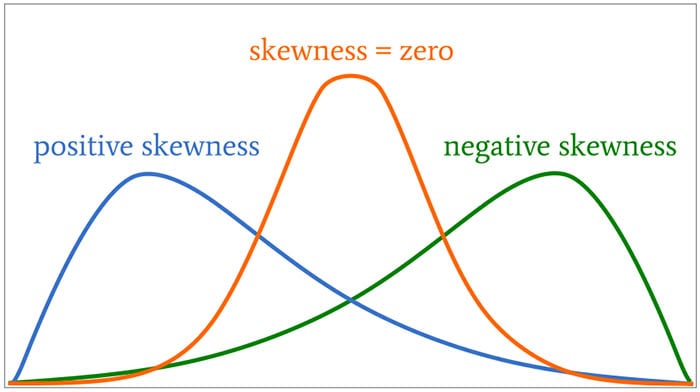
Depiction of positive skewness, skewness, and negative skewness.
Skewness can be a positive or negative number (or zero). Distributions that are symmetrical with respect to the mean, such as the normal distribution, have zero skewness. A distribution that “leans” to the right has negative skewness, and a distribution that “leans” to the left has positive skewness.
As a general guideline, skewness values that are within ±1 of the normal distribution’s skewness indicate sufficient normality for the use of parametric tests.
Kurtosis
We use kurtosis to quantify a phenomenon’s tendency to produce values that are far from the mean. There are various ways to describe the information that kurtosis conveys about a data set: “tailedness” (note that the far-from-the-mean values are in the distribution’s tails), “tail magnitude” or “tail weight,” and “peakedness” (this last one is somewhat problematic, though, because kurtosis doesn’t directly measure peakedness or flatness).
The normal distribution has a kurtosis value of 3. The following diagram gives a general idea of how kurtosis greater than or less than 3 corresponds to non-normal distribution shapes.
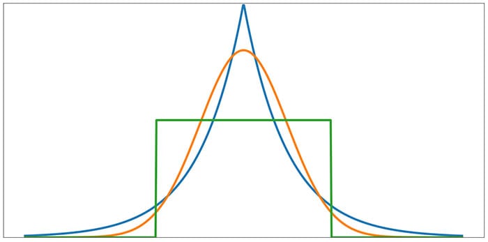
Notice that kurtosis greater than or less than 3 corresponds to non-normal distribution shapes.
The orange curve is a normal distribution. Notice how the blue curve, compared to the orange curve, has more “tail magnitude,” i.e., there is more probability mass in the tails. The kurtosis of the blue curve, which is called a Laplace distribution, is 6. The green curve is called the uniform distribution; you can see that the tails have been eliminated. The kurtosis of the uniform distribution is 1.8.
As with skewness, a general guideline is that kurtosis within ±1 of the normal distribution’s kurtosis indicates sufficient normality.
Conclusion
There is certainly much more we could say about parametric tests, skewness, and kurtosis, but I think that we’ve covered enough material for an introductory article. Here’s a recap:
- We favor parametric tests when measurements exhibit a sufficiently normal distribution.
- Skewness quantifies a distribution’s lack of symmetry with respect to the mean.
- Kurtosis quantifies the distribution’s “tailedness” and conveys the corresponding phenomenon’s tendency to produce values that are far from the mean.