Technical Article

The Cumulative Distribution Function in Normally Distributed Data

August 19, 2020 by Robert Keim

This article explains how we obtain the Gaussian cumulative distribution function and why it is useful in statistical analysis.

If you're just joining us in this discussion on statistics and electrical engineering, it may be helpful to first review the past articles in the series:

Here's what we know from previous articles:

We can create a probability density function of normally distributed measurements by computing the standard deviation and mean of the data set.
This probability density function is an idealized mathematical equivalent of the shape that we observe in the data set’s histogram.
We obtain probability—i.e., the likelihood that certain measurement values will occur—by integrating the probability density function over a specified interval.

If integrating portions of the probability density function is the key to extracting probabilities from measured data, one might wonder about the possibility of simply integrating the entire function and thereby producing a new function that gives us direct access to probability information.

As it turns out, this is a standard technique in statistical analysis, and this new function that we obtain by integrating the entire probability density function is called the cumulative distribution function.

The Cumulative Normal Distribution Function

Using a cumulative distribution function (CDF) is an especially good idea when we’re working with normally distributed data because integrating the Gaussian curve is not particularly easy.

In fact, in order to create the CDF of the Gaussian curve, even mathematicians must resort to numerical integration—the function $e^{-x^2}$ does not have an antiderivative that can be expressed in elementary form. This means that the Gaussian CDF is actually a sequence of discrete values generated from numerous individual samples taken along the Gaussian curve.

In the age of computers, we can easily process an immense number of samples, and consequently, the discrete CDF produced by numerical integration can be a perfectly adequate replacement for a continuous function obtained via symbolic integration.

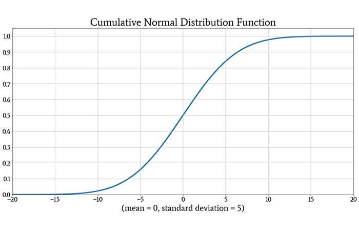
If we plot a large number of values in the Gaussian CDF, the curve looks like this:

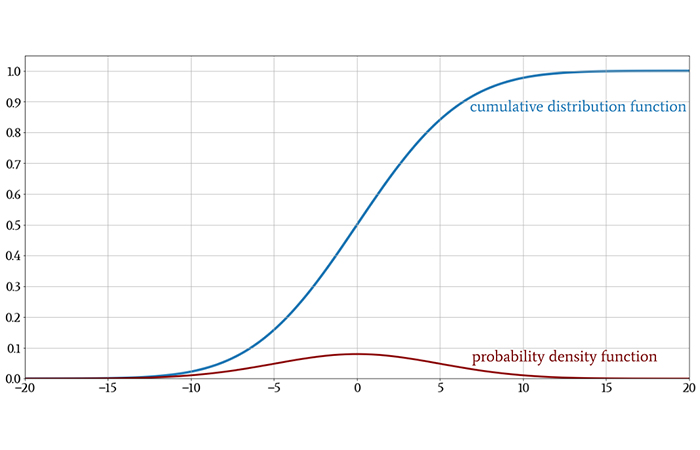
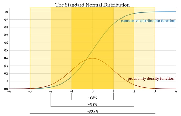
The following plot shows both the original Gaussian probability density function and its CDF, so that you can get a feeling for how integration turns one into the other.

One quick note before we move on: You may see the symbol Φ (the uppercase Greek letter phi) in statistical discussions. When a normal distribution has a mean of 0 and a standard deviation of 1, it is called the standard normal distribution. The CDF of the standard normal distribution is denoted by Φ; thus,

$$\Phi(z)=\frac{1}{\sqrt{2 \pi}}\int_{-\infty}^{z}e^{-\frac{x^2}{2}}dx$$

Example of the Cumulative Distribution Function

When we integrate a probability density function from negative infinity to some value denoted by z, we are computing the probability that a randomly selected measurement, or a new measurement, will fall within the numerical interval that extends from negative infinity to z. In other words, we are computing the probability that the measured value will be less than z.

This is exactly the information that we obtain from the CDF and without the need for integration. If we look at the CDF and find the vertical value corresponding to some number z on the horizontal axis, we know the probability that a measured value will be less than z.

For example:

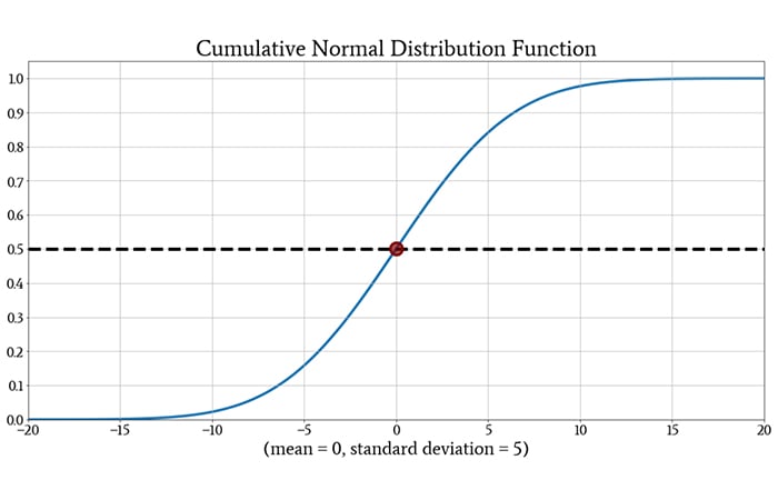
The CDF has a value of 0.5 at z = 0. This tells us that a randomly selected measurement has a 50% chance of being less than zero. This result makes intuitive sense: the normal distribution is symmetric with respect to the mean, and since the mean is zero in this case, any individual measurement has an equal chance of being less than or greater than zero.

The CDF also provides a straightforward way of determining the probability that a measurement will fall within a specific range. If the range is defined by the two values z₁ and z₂, all we need to do is subtract the value of the CDF at z₂ from the value of the CDF at z₁ (and then take the absolute value if necessary).

Here’s another example:

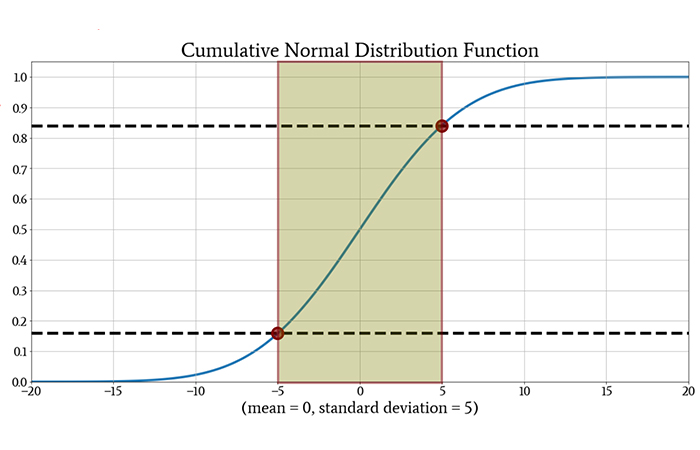
The probability that a randomly selected measurement will be between –5 and +5 is approximately 0.84 – 0.16 = 0.68 (or 68%). The more precise value is 68.27%.

Probabilities and Standard Deviation

You might have noticed that the interval chosen in the preceding example was equal to one standard deviation above and below the mean. When we discuss probabilities with reference to intervals reported in units of standard deviation, the information applies to all data sets that follow the normal distribution. Thus, we can specify probability characteristics using the CDF of the standard normal distribution, and then extend these trends to other data sets simply by changing the standard deviation (or by thinking in terms of standard deviations).

We saw above that in normally distributed data, a measured value has a 68.27% chance of falling within one standard deviation of the mean. We can continue summarizing normally distributed data as follows:

The probability that a measured value will be within two standard deviations of the mean is 95.45%.
The probability that a measured value will be within three standard deviations of the mean is 99.73%.

These three probabilities provide a simple overview of how normally distributed measurements will behave.

A more approximate version of this summary is known as the 68-95-99.7 rule: if a data set exhibits a normal distribution, about 68% of the values will be within one standard deviation of the mean, about 95% will be within two standard deviations, and about 99.7% will be within three standard deviations.

Conclusion

We’ve covered some important material, and I hope that you’re enjoying our exploration of the normal distribution and related statistical topics. In the next article, we’ll look at two not-so-widely-known descriptive statistical measures: skewness and kurtosis.