The Normal Distribution: Understanding Histograms and Probability

This article is part of a series on statistics in electrical engineering, which we kicked off with our discussion of statistical analysis and descriptive statistics. Next, we explored three descriptive statistical measures from the perspective of signal-processing applications.

We then touched on standard deviation—specifically, determining sample-size compensation when calculating standard deviation and understanding the relationship between standard deviation and root-mean-square values. 

In the last article, we introduced normal distribution in electrical engineering, laying the groundwork for our present discussion:  understanding probabilities in measured data.

 

Understanding Histograms

In the previous article, we started our discussion of the normal distribution by referring to the shape of this histogram:

 

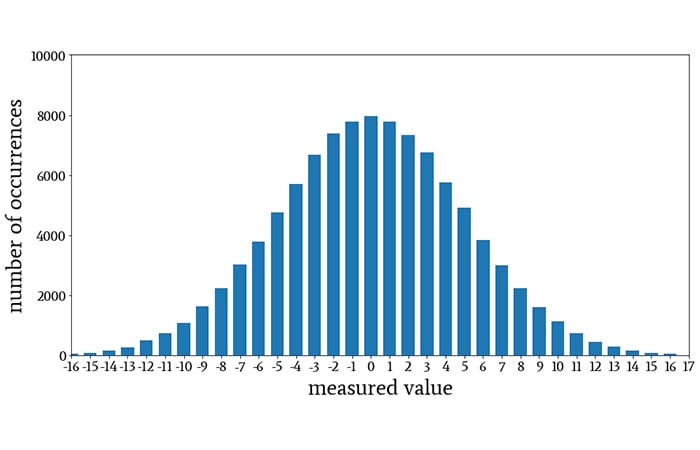
A histogram illustrating normal distribution.

 

I think that most people who work in science or engineering are at least vaguely familiar with histograms, but let’s take a step back.

What exactly is a histogram?

Histograms are visual representations of 1) the values that are present in a data set and 2) how frequently these values occur. The histogram shown above could represent many different types of information.

Let’s imagine that it represents the distribution of values that we obtained when measuring the difference, rounded to the nearest millivolt, between the nominal and actual output voltage of a linear regulator that was subjected to varying temperatures and operational conditions. Thus, for example, approximately 8,000 measurements indicated a 0 mV difference between the nominal output voltage and the actual output voltage, and approximately 1,000 measurements indicated a 10 mV difference.

Histograms are extremely effective ways to summarize large quantities of data. By glancing at the histogram above, we can quickly find the frequency of individual values in the data set and identify trends or patterns that help us to understand the relationship between measured value and frequency.

 

Histograms with Bins

When a data set contains so many different values that we cannot conveniently associate them with individual bars in a histogram, we use binning. That is, we define a range of values as a bin, group measurements into these bins, and create one bar for each bin.

The following histogram, which was generated from normally distributed data with a mean of 0 and a standard deviation of 0.6, uses bins instead of individual values:

 

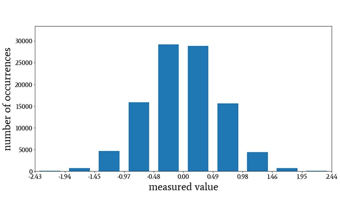
A histogram using bins instead of individual values.

 

The horizontal axis is divided into ten bins of equal width, and one bar is assigned to each bin. All of the measurements that fall within a bin’s numeric interval contribute to the height of the corresponding bar. (The labels on the horizontal axis indicate that the bins are not of equal width, but that’s just because the label values are rounded.)

 

Histograms and Probability

In some situations, the histogram doesn’t give us the information that we want. We can look at a histogram and easily determine the frequency of a measured value, but we cannot easily determine the probability of a measured value.

For example, if I look at the first histogram, I know that approximately 8,000 measurements reported a 0 V difference between the nominal and actual voltage of the regulator, but I don’t know how likely it is that a randomly selected measurement, or a new measurement, will report a 0 V difference.

This is a serious limitation because probability answers the extremely common question, What are the chances that …?

What are the chances that my linear regulator will have an output-voltage error of less than 2 mV? What are the chances that my data link’s bit error rate will be higher than 10^–3? What are the chances that noise will cause my input signal to exceed the detection threshold? And so forth.

The origin of this limitation is simply that the histogram does not clearly convey the sample size, i.e., the total number of measurements. (In theory, the total number of measurements could be determined by adding the values of all the bars in the histogram, but this would be tedious and imprecise.)

If we know the sample size, we can divide the number of occurrences by the sample size and thereby determine the probability. Let’s look at an example.

 

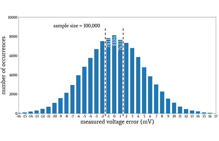
Example of how a histogram can help us determine probability by dividing the number of occurrences by the sample size.

 

The red dashed lines enclose the bars that report voltage errors less than 2 mV, and the numbers written inside the bars indicate the exact number of occurrences for those three error voltages. The sum of those three numbers is 23,548. Thus, based on this data-collection exercise, the probability of obtaining error of less than 2 mV is 23,548/100,000 ≈ 23.5%.

 

The Probability Mass Function

If our primary objective in creating a histogram is to convey probability information, we can modify the entire histogram by dividing all the occurrence counts by the sample size.

The resulting plot is an approximation of the probability mass function. For example:

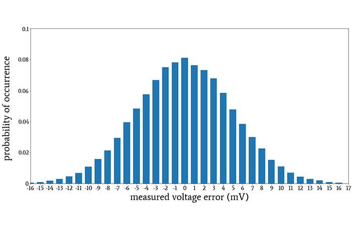
A histogram depicting the approximate probability mass function, found by dividing all occurrence counts by sample size.

 

All we’ve really done is change the numbers on the vertical axis. Nonetheless, now we can look at an individual value or a group of values and easily determine the probability of occurrence.

I want to clarify the following detail: I said that we approximate the probability mass function when we take a histogram and divide the counts by the sample size. A true probability mass function represents the idealized distribution of probabilities, meaning that it would require an infinite number of measurements.

Thus, when we’re working with realistic sample sizes, the histogram generated from measured data gives us only an approximation of the probability mass function.

 

Probability Mass vs. Probability Density

It’s worth emphasizing that the probability mass function is the discrete equivalent of the probability density function (which we discussed in the previous article).

Whereas the probability density function is continuous and provides probability values when we integrate the function over a specified range, the probability mass function is discretized and gives us the probability associated with a specific value or bin.

These two functions convey the same general statistical information about a variable or waveform, but they do so in different ways.

Note the difference between the two names: The vertical axis of a probability mass function indicates the mass, as in the amount, of probability. The vertical axis of a probability density function indicates the density of probability relative to the horizontal axis; we have to integrate this density along the horizontal axis in order to generate an amount of probability.

 

Conclusion

We’ve covered probability mass and density functions, and now we’re ready to study the cumulative distribution function and to examine normal-distribution probabilities from the perspective of standard deviation. These will be our topics for the next article.