Introduction to Histogram Equalization

In a previous article, we saw that it is possible to adjust image contrast by modifying the slope of the mapping function.

In this article, we’ll look at another contrast enhancement technique often referred to as histogram equalization. We’ll explain the basic idea of this important technique and introduce its mapping function which is obtained from the image histogram information.

 

What Is an Image Histogram?

An image histogram is a plot that gives the number of occurrences of the different pixel values in the image. Histograms are extensively used to enhance images or extract useful information from them. Figure 1 shows an eight-bit grayscale image.

 

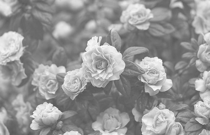
Figure 1. Image courtesy of Favim.com 

 

The histogram of this image is shown in Figure 2.

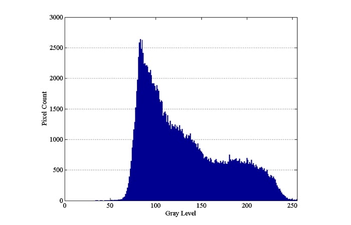
Figure 2

 

The x-axis of an image histogram shows the pixel intensities. For the eight-bit example shown in Figure 2, there are a total of 256 different pixel values (the x-axis ranges from 0 to 255). The y-axis of the histogram specifies the number of pixels for a given pixel value. Each of the possible values of the histogram x-axis is referred to as a bin of the histogram.

While the histogram in Figure 2 has the maximum possible number of bins for an 8-bit grayscale image, we sometimes prefer to reduce the number of bins. In this case, we combine the adjacent values of the x-axis and represent them as a single bin.

Note that the above image does not have the darkest shades of gray. That’s why the histogram shows a small number of pixels below a gray level value of about 60. In fact, the histogram shows that the number of occurrences of the pixel values close to 80 are much greater than the other values. 

 

Contrast Adjustment

Figure 3 shows a close-up of the histogram at lower gray level values. 

 

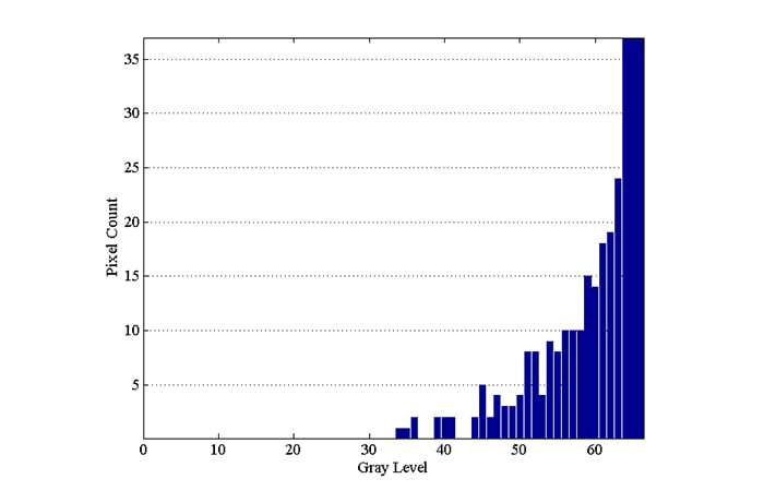
Figure 3

 

The histogram shows that there is no pixel with a value less than or equal to 33. This means that 34 out of the total 256 different pixel values of an 8-bit image are not used in this example. Hence, we can apply a contrast adjustment mapping so that the pixel values 34 and 255 get mapped to 0 and 255, respectively. This will stretch the pixel values of the image to occupy the full range of available values and will improve the viewability of the image.

Figure 4(b) shows the contrast-adjusted image. To make the comparison more convenient, the original image is shown in Figure 4(a), as well.

 

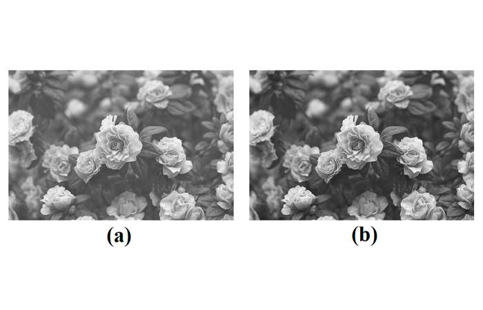
Figure 4. (a) The original image and (b) contrast-adjusted version.

 

The histogram of the modified image is shown in Figure 5. 

 

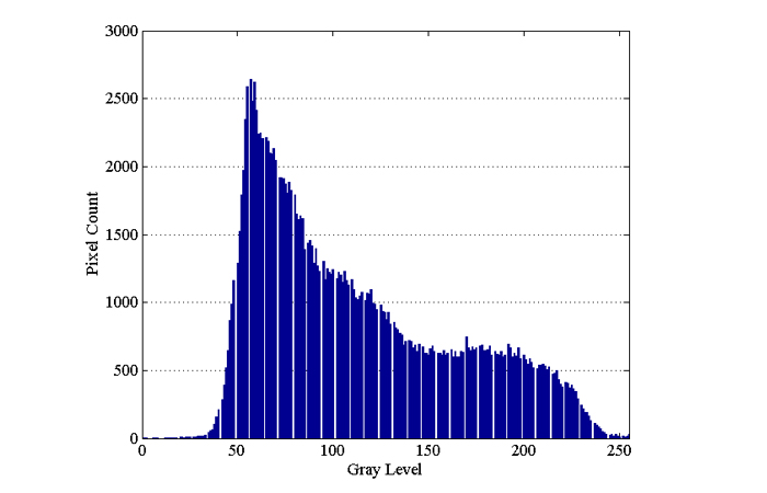
Figure 5

 

The Basic Idea of Histogram Equalization

In the above example, the pixel values below 34 were not at all present in the image. We were able to adjust the contrast by mapping the minimum pixel value of the image to the lowest value of the available range, i.e., zero.

Can we further enhance the contrast of this image?

Figure 3 shows that, although the minimum pixel value is 34, there is only one pixel with this value! In fact, the pixel values between 34 and 44 appear less than or equal to two times in the whole image which consists of 167000 pixels. The number of occurrences of the pixel values between 45 and 58 is not large either (less than 10 times).

Although the pixel values between 34 and 44 are rare and might be even negligible in this example, the contrast adjustment of the previous section takes them into account and maps the range 34 to 255 to the range 0 to 255. In other words, this method only considers the minimum and the maximum pixel values no matter how many times they appear in the image.

If we could take the number of occurrences of the different pixel values into account, we might be able to achieve a better contrast. For example, consider a hypothetical transfer function that maps the pixel values around the peak of the histogram—shown by the blue arrow in Figure 6—to the range shown by the green arrow.

 

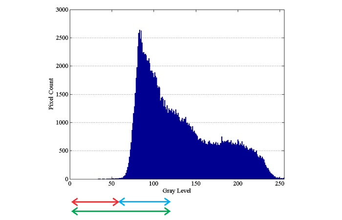
Figure 6

 

Since the pixel values around the histogram peak are mapped to a wider range the contrast of these regions will be improved. However, this will probably lead to loss of information (or contrast degradation) in the pixels that correspond to the range shown by the red arrow. This is due to the fact that we are mapping some of the pixel values around the histogram peak to the range shown by the red arrow while the original image already had some pixels in this range.

To summarize, such a contrast enhancement method can improve the overall contrast of the image because it stretches the pixel values around the histogram peak that is related to the majority of the pixel values in the image.

However, it can reduce the contrast in the regions of the image that correspond to the less frequent pixel values. After applying this method, we should get a flatter histogram because some of the pixels of the histogram peak are mapped to the pixel values that are less frequent.  

 

How to Achieve Better Histogram Equalization

The concept discussed above is the basic idea behind a contrast enhancement method called “histogram equalization”. The histogram equalization technique achieves contrast improvement by spreading the more frequent pixel values over those pixel values that have a smaller number of occurrences.

After applying this technique, the image histogram should be flatter than the original histogram.

Figure 7(c) shows the result of applying this technique to our example image. Figure 7(a) and 7(b) are respectively the original image and the result of the previous contrast enhancement method (from Figure 4) that are reproduced for the sake of comparison.

 

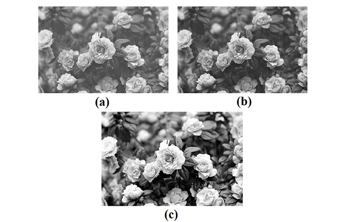
Figure 7. (a) The original image, (b) the results of the initial contrast enhancement method, and (c) the results of the new method.

 

The histogram of Figure 7(c) is shown in Figure 8.

 

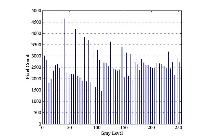
Figure 8

 

While the histogram of the original image (Figure 2) has a small number of pixels at below a gray level of about 58, the gray level distribution of the new image is almost uniform.

What mapping function should we apply to make the image histogram (almost) uniform?

It can be shown that such a mapping function can be obtained from the histogram of the input image. Assume that the number of occurrences of the pixel value x_k in the input image is n_k (as shown in Figure 9). 

 

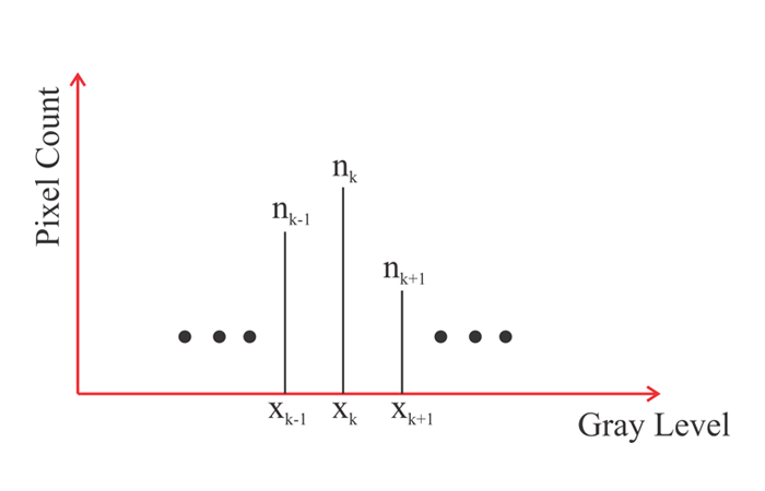
Figure 9

 

To equalize this histogram, we should map the pixel value x_k to y_k given by the following equation:

 

\[y_k=(L-1)\sum_{j=0}^k \frac {n_j}{N}\]

 

where L is the total number of possible gray levels (e.g. L=256 for an 8-bit image) and N is the total number of pixels in the image. 

In the next article of this series, we’ll try to develop intuition into how the above mapping function can flatten the image histogram. We’ll also examine the circuit implementation of this technique.  

 

Conclusion

A contrast adjustment mapping can be used to stretch the pixel values of a given image to occupy the full range of available values. This method considers the minimum and the maximum pixel values of the image even if they appear only once in the image.

In contrast, the histogram equalization method takes the number of occurrences of the different pixel values into account and attempts to flatten the image histogram. This method can improve the overall contrast of the image at the cost of reducing the contrast in the regions of the image that correspond to the less frequent pixel values. 

The next article in this series will look at the mapping function in greater detail and examine the circuit implementation of this technique. 

 

To see a complete list of my articles, please visit this page.