An Intro to Adaptive Echo Cancellers

This article introduces a basic acoustic echo canceller based on the Least Mean Squares (LMS) algorithm. Acoustic echo cancellers are necessary for many modern communications products.  I’m sure you’ve come across a time when you could hear your voice while speaking on the phone, correct? Well, that's an example of an acoustic echo. Acoustic echoes are a common problem that arise from audio signals bouncing off nearby objects and coupling into the microphone when the mic should only be picking up your voice or when directly coupling from a speaker microphone pair (like your phone). Without cancelling these effects, the communication system is pretty annoying to use!

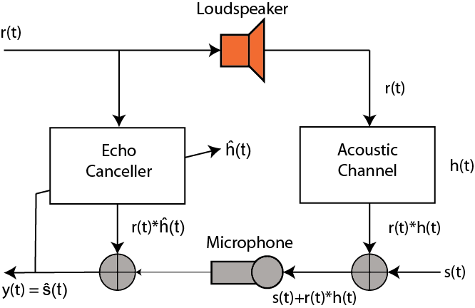
Figure 1

Here, the speech signal from a loudspeaker is acoustically coupled into the microphone of a speaker phone or hands-free cell phone, which is heard at the remote signal source as a return echo. The echo is suppressed by an echo canceller at the echo source by the system modeled in the figure above. Assume the channel has the sampled data impulse response represented by the Z-transform:

$$H(Z) = 1 + 0.5Z^{-3} + 0.1Z^{-5}$$   

and the echo canceller is a tapped delay filter of length 50 samples. First we will let the desired signal s(t) be zero and train the canceling filter with white noise. As a synopsis, the signals in the figure 1 are:

$$\text{speech signal}: s(t)$$

$$\text{echo}: r(t)$$

$$\text{acoustic channel}: h(t)$$

$$\text{acoustic channel output} = r(t)*h(t) \text{(convolution)}$$

$$\text{microphone input}: s(t) + r(t)*h(t) , \text{desired signal plus echo through acoustic channel}$$

$$\text{echo canceller}: \hat{h}(t)$$

$$\text{desired signal}: y(t)$$

The goal is to match the acoustic channel with our echo canceller so that we can invert the acoustic channels response and create only the desired signal at the microphone inputs (t). So lets see how this looks in Matlab code:

clear all;
clf;
close all;

%acoustic channel frequency response
num = [1 0 0 0.5 0 .1];
den = [1 0 0  0 0 0];
[Hc,Wc] = freqz(num,den);

%---BUILD FM SWEEP---%
fs = 2*pi;
tmax = 10000;

f1=0;
f2 = .5;
tsweep = 0:499;
slope = (f2-f1)/1000;
F = slope.*(mod(tsweep,500));

t = 0:1:tmax;
fm = cos(2*pi*slope*t);


F = slope.*(mod(tsweep,500));
fm2 = cos(2*pi*(F).*tsweep);
fm2c = repmat(fm2,20,1);
fm2 = reshape(fm2c',1,10000 );

figure
plot([0:999],fm2(2001:3000))
%subplot(212)
%plot([-512:511]*1/(2*pi), 20*log10(abs(fft(fm2(1:500), 1024))))
grid on
%End building of FM sweep

trainlen = tmax;



%training signal
r_t = 1*rand(1,tmax);

%desired signal
s_t = 0;

%signal through channel
rt_ht = filter(num,den,r_t);

%signal through channel + desired
mic_in = s_t + rt_ht;

%LMS algorithm of echo canceller
reg1=zeros(1,50);
wts = (zeros(1,50));
mu  = .07;
for n = 1:trainlen
 
  wts_sv = wts;
 
  reg1 = [r_t(n) reg1(1:49)];
 
  err = mic_in(n) - reg1*(wts');
 
  y(n) = err;
 
  wts = wts + mu*(reg1*(err'));
   
end

%plots
figure
subplot(211)
plot(1:length(y), (y))
hold on
plot(1:10000, zeros(1,10000), 'color', 'r', 'linewidth', 2, 'MarkerSize', 2)
hold off
axis([ -.5 10000 -1 1.1])
grid on
title('Steady State (time response) Desired Signal = 0, trained with white noise')
subplot(212)
plot(1:length(y), 20*log10(abs(y)))
grid on
title('Log Magnitude Training Curve, trained with white noise')



[Hf,Wf] = freqz(wts_sv);
figure
subplot(211)
plot(Wc/pi, 20*log10(abs(Hc)))
grid on
title('Frequency Response of Channel')
subplot(212)
plot(Wf/pi, 20*log10(abs(Hf)),'color','r')
title('Frequency Response of Adaptive Canceller, trained with white noise')
grid on



Adaptive_Echo_Canceler_.zip

In the code, we first add the acoustic channel response into the Hc and Wc variables. Then we build an FM sweep training signal for use in the second part of training the echo canceller. We then define the signals r_t, s_t, Ort_ht, and mic_in to reflect Figure 1. Now comes the bulk of the adaptive canceller: we train it with a simple iterative least mean squares approach.

First, we define a register of depth 50. This is analogous to an array in C or C++ (embedded application). We then define an empty array of weights--wts--and set the $$\mu$$, which is an important stepping factor in the least mean squares algorithm which takes tiny steps each iteration to find the optimal set of weights which describe the acoustic channel and give the smallest error for each input. The LMS algorithm is simple-- we first add a sample of white noise to the register, then calculate the error:

$$err = \text{mic_in}(n) - reg1*wts'$$

and then update the weights

$$wts = wts + \mu*(reg1*err')$$

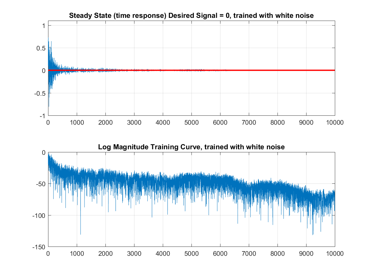
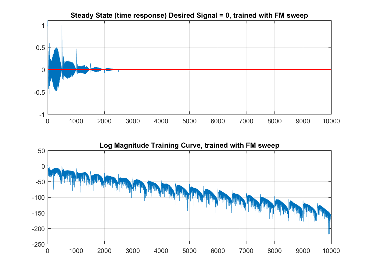
The derivation of the weight update is a long-winded explanation which I will not get into in this article, but will post a separate explanation of soon. However, the update reduces to the current weights plus $$\mu$$ times the contents of the register times the transpose of the error. Letting this run until convergence, we see that our algorithm finds the ultimate set of weights when trained on white noise to reach the desired signal of 0. 

 

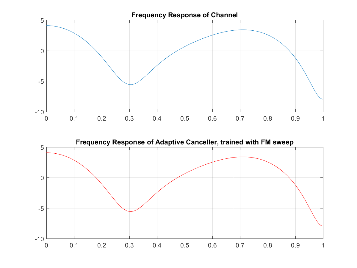
And we can see the echo canceller response converges almost exactly to the acoustic channels frequency response.

 



Now if we train it without the FM signal, we see it converges a little slower, but the error is magnitudes smaller!

 





 

And that's it--a pretty decent echo canceller in a couple lines of code. Look out for the Least Mean Squares article for a more thorough investigation into how the algorithm works!