Finding Summary Statistics and Probabilities with the Binomial Distribution

If you’ve read the previous article, you know that the binomial distribution is a tool that facilitates statistical analysis in scenarios that occur frequently in engineering and other fields. After confirming that your analytical situation meets the requirements of the binomial distribution, you need to identify the number of trials and the probability of success. Now you’re ready for action.

 

Calculating Mean

The mean (μ) of a binomially distributed random variable is equal to the number of trials (n) multiplied by the probability of success (p):

 

$$\mu=np$$

 

This makes intuitive sense if we consider a coin toss. Let’s define heads as a success. We know that the probability of success is 50%, or 0.5 (remember that we need to use the decimal form when doing calculations). If you flip a coin 20 times, the expected number of successes—i.e., the mean—is 20 × 0.5 = 10.

 

Calculating Standard Deviation

The standard deviation (σ) of a binomially distributed random variable also depends only on the number of trials and the probability of success. This relationship is a bit more complicated, though:

 

$$\sigma=\sqrt{np(1-p)}$$

 

You might also see (1-p) written as q, which denotes the probability of failure.

 

$$\sigma=\sqrt{npq}$$

 

If you prefer to work with variance, just remove the square root sign:

 

$$\sigma^2=np(1-p)$$

 

Calculate Probability—Probability Distribution Function and Cumulative Distribution Function

When we’re dealing with probabilities in a binomial setting, it helps to be a bit more formal with our notation and terminology. After examining your analytical scenario, you need to define a random variable. We’ll use the letter X (statisticians use uppercase letters when defining a random variable).

Let’s go back to the coin toss example. We define our random variable as follows: Let X = the number of heads obtained by flipping a fair coin 100 times. We know that n = 100 and p = 0.5. A quick calculation gives us μ = 50 and σ = 5.

There are three basic types of probability questions that we can ask:

1. What is the probability that X will equal a given number?
2. What is the probability that X will be less than or equal to a given number?
3. What is the probability that X will be greater than or equal to a given number?

In probability notation, we use the lowercase version of the random variable’s letter to represent a specific value of the random variable. Thus, x replaces “a given number,” and we can concisely express these three questions as follows:

• P(X = x) = ?
• P(X ≤ x) = ?
• P(X ≥ x) = ?

To answer question #1, we use the binomial probability distribution function (pdf). If we were dealing with a continuous probability density function, P(X = x) would always be zero. The binomial setting, however, involves discrete trials. X assumes integer values, not a continuous range of values, and therefore we can assign a nonzero probability to P(X = x).

For questions #2 and #3, we use the binomial cumulative distribution function (cdf). The cumulative distribution function is the integral of the probability distribution function, allowing us to easily calculate the probability associated with a range of possible values. The tedious alternative is to use the pdf and add up all the probabilities associated with each value in the specified range.

Nowadays, we rely on technology to extract the required information from pdf and the cdf. A TI graphing calculator can do the job, but most people will probably prefer to use an online tool such as the University of Iowa’s binomial distribution applet, shown in Figure 1:

 

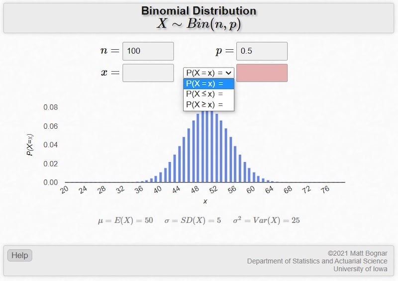
Figure 1. Binomial distribution example where n = 100 and p = 0.5. Screenshot used courtesy of the University of Iowa and Matt Bognar

 

Thanks to the University of Iowa for this straightforward, visually appealing tool.

With this applet, you input n, p, and x. It gives you the mean, standard deviation, and variance calculates the three types of probabilities discussed above, and displays the probability distribution function. Figure 1 shows results for a scenario involving 100 coin tosses.

 

Applying the Binomial Distribution to an Engineering Problem

Let’s work through an example. 

You’re testing a PCB that occasionally experiences a firmware failure within a few seconds after power-up. Through extensive observation, you determine that the failure occurs about once for every 17 power-ups. The failures seem to occur randomly and to have no effect on the likelihood of a failure in subsequent power-ups. 

You need to take the board out for field testing, and you don’t have time to find what has proved to be an elusive bug. You’re hoping that the issue won’t seriously interfere with the field test, which will require the board to be powered up and then power cycled twice, meaning three power-ups.

You decide to use statistical analysis to assess the situation. More specifically, you ask the following questions:

1. What is the probability that the board will fail at least once during the field test?
2. What is the probability that the board will fail after all three power-ups?

 

The Solution—Success in Failures

In this scenario, we have three trials (each power-up in the field-testing sequence is a trial), and the probability of success is p = 1 ÷ 17 ≈ 0.059. (Note that “success” in this example is a failure! I warned you about this sort of thing in the first article.) The average number of failures per field test is μ = np = (3)(0.059) ≈ 0.18.

Here (Figure 2) is the answer to question #1:

 

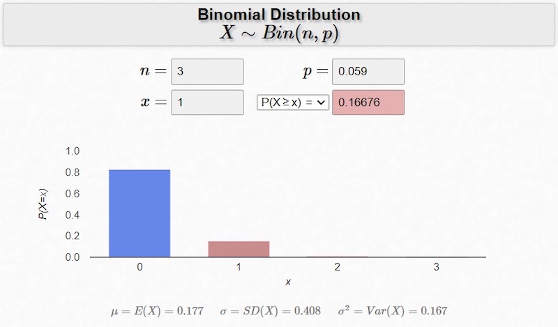
Figure 2. Binomial distribution example where n = 3, p = 0.059, and x = 1. Screenshot used courtesy of the University of Iowa and Matt Bognar

 

So there’s a 17% chance that your board will fail at some point during the field test. For me, 17% likelihood would be sufficient to cause significant anxiety if this were a high-visibility test.

Next, Figure 3 shows the answer to question #2:

 

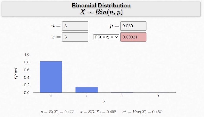
Figure 3. Binomial distribution example where n = 3, p = 0.059, and x = 3. Screenshot used courtesy of the University of Iowa and Matt Bognar

 

With P(X = 3) = 0.02%, we can be very confident that at least your colleagues won’t conclude that your board does little more than consistent malfunction.

I hope that you now have a clear idea of how we apply the binomial distribution to a real-life problem that calls for statistical analysis. We’ll look at more examples in the next article.