Understanding the t-Distribution in Tests for Statistical Significance

This article is a continuation of Robert Keim's series on statistics in electrical engineering. If you've been following along, feel free to skip to the section below for a brief recap of statistical significance. If you're just joining in, please review earlier articles in the series: 

1. The role of statistical analysis in electrical engineering
2. The role of descriptive statistics in electrical engineering
3. Average deviation, standard deviation, and variance in signal processing
4. Understanding sample-size compensation in standard deviation calculations
5. Introduction to the normal distribution in electrical engineering
6. Understanding histograms and probability
7. What is the cumulative distribution function in normally distributed data?
8. Parametric tests, skewness, and kurtosis
9. Finding statistical relationships with correlation, causation, and covariance
10. Using correlation coefficients to find statistical relationships
11. Statistical significance in experimentation and data analysis

 

A Quick Review of Statistical Significance

The previous article explored the concept of statistical significance, which provides a widely used—though potentially misleading—technique for deciding whether a relationship exists between experimental variables. Here’s a recap:

• An experiment involves two (or more) variables that may be related in some way. The null hypothesis states that there is no relationship between these variables.
• Usually, we hope that an experiment will disprove the null hypothesis. In other words, we have reason to believe that two variables are related in some way, and we design an experiment with the intention of collecting data that demonstrate the existence of a relationship.
• We can calculate the probability of obtaining an observed value, or a more extreme value, under the assumption that the null hypothesis is true. This is called the p-value. It conveys the likelihood of obtaining a value that is at least as extreme as the observed value given that no relationship exists between experimental variables.
• Statistical significance is determined by comparing the p-value to a predetermined threshold called the significance level, denoted by ⍺. Common significance levels are 1% (⍺ = 0.01) and 5% (⍺ = 0.05).
• If the p-value is less than the significance level, we are justified in rejecting the null hypothesis. In other words, we can claim that a relationship exists, because if the experimental variables were indeed unrelated, we probably would not have obtained the observed value.

My objective in this article is to cover essential information about a distribution that plays an important role in tests of statistical significance, and in the next two articles, we’ll discuss t-values and work through a simple example of statistical significance applied to engineered systems.

 

The t-Distribution

The null hypothesis often takes the form of a normal distribution, because that’s the distribution of values produced by so many phenomena that are influenced in random or extremely complex ways. However, when we actually need to calculate a p-value and report statistical significance, we very frequently use the t-distribution.

The t-distribution is similar to the normal distribution, and as sample size increases it gradually becomes identical to the normal distribution. The term “t-distribution” actually refers to a family of distribution curves, because the curve changes according to the experiment’s sample size.

More specifically, the exact shape of a t-distribution is determined by a parameter called degrees of freedom, denoted by \( \nu \) (this is the lowercase Greek letter nu, not Latin v). Degrees of freedom is equal to the sample size (denoted by n) minus one:

 

\[\nu=n-1\]

 

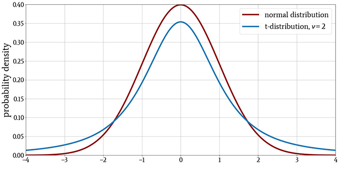
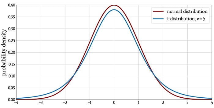
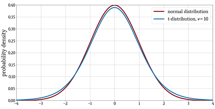
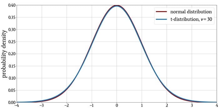
The following plots show the t-distribution for different values of \( \nu \), with the normal distribution included for comparison.

 

Characteristics of the t-Distribution

The t-distribution resembles the standard normal distribution: its mean is zero, it is symmetric about the mean, and the probability density decreases with the same general curvature for values above and below the mean.   

As you can see in the plots, the t-distribution has more probability density in the tails and less in the region near the peak. This tells us that the t-distribution, in comparison to the normal distribution, produces more values that are far from the mean.

However, this difference diminishes as ν increases, indicating that a larger sample size reduces the tendency to observe values that are far from the mean. The last plot demonstrates that when the distribution has more than approximately 30 degrees of freedom, there is essentially no difference between the t-distribution and the normal distribution.

 

The Origin of the t-Distribution

A concept that is closely related to statistical significance is the confidence interval. The following diagram illustrates the two-sided 95% confidence interval of a standard normal distribution.

 

     

 

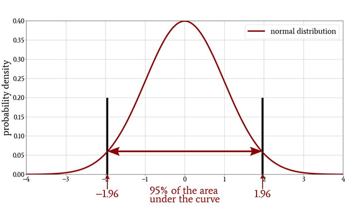
If the mean of a sample—that is, the mean of the measurements that we gathered during an experiment—falls within this confidence interval, the observed values are not statistically significant at a significance level of 5%. The sample mean must fall outside of the confidence interval in order to justify rejection of the null hypothesis.

The two values that define the confidence interval are called the critical values. In the case of a standard normal distribution, the critical values for a two-sided 95% confidence interval, which corresponds to a significance level of 5%, are –1.96 and +1.96. The critical values will change if we choose a different significance level.

It turns out that when the sample size in an experiment is small, the confidence interval will be too narrow if we model the null hypothesis as a normal distribution. This means that some observed values could fall outside the interval and therefore suggest statistical significance when in reality the experimental result is not statistically significant.

Why is the confidence interval too narrow when we use the normal distribution?

A full explanation would be too long for this article, but the problem boils down to the fact that we do not know the standard deviation of the population and must use the standard deviation of the sample instead. The standard deviation of a very small sample seriously underestimates the actual standard deviation, and we use the t-distribution to compensate for this effect.

As sample size increases, less compensation is required, and this is why the t-distribution more closely resembles the normal distribution when we have a larger sample size.

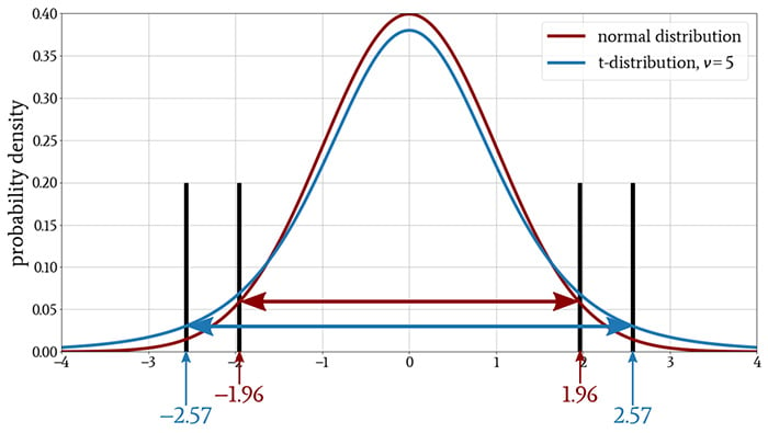
As you can see in the following plot, the 95% confidence interval becomes wider when we use the t-distribution instead of the normal distribution.

 

Conclusion

At this point, our discussion of the t-distribution is still quite theoretical. I hope that it has been theoretical in a good way, but in any event, future articles will help you to understand how we convert some of this theory into practice.