Technical Article

Finding Statistical Relationships: Correlation, Causation, and Covariance

September 16, 2020 by Robert Keim

This article explains a statistical measure that helps us to draw conclusions about how one variable affects another.

In this series on statistics in electrical engineering, All About Circuits Director of Engineering Robert Keim breaks down high-level definitions and examples of statistics concepts that can be applied in the design process. You can catch up on the articles so far in the following list or skip to the "Correlation and Causation" section below.

Correlation and Causation

Let’s say that we have a wireless communication system that is giving us trouble. The bit error rate (BER) changes dramatically from one field test to the next, and there is no obvious cause for this unstable behavior. To make matters worse, the field tests are not even close to controlled experiments, and there are quite a few factors—thermal and atmospheric conditions, vibration, RF interference, EMI from nearby equipment, orientation, relative velocity—that could be affecting the system’s performance.

One way of dealing with this situation is to choose the factors that are most likely to heavily influence BER, gather some data, and look for causal relationships. Since it is often very difficult to prove causality, our analysis will actually quantify correlation, and then we can either assume that correlation indicates causation (which is risky) or attempt to demonstrate causation by collecting new data from a carefully designed experiment.

Thus, the search for causation begins with the search for correlation, and correlation begins with covariance.

Variables That Vary Together

The descriptive statistical measure called variance is discussed in a previous article that also covers standard deviation. Variance (denoted by σ²) is the averaged power, expressed in units of power, of the random deviations in a data set. We calculate variance as follows:

\[\sigma^2=\frac{1}{N-1}\sum_{i=1}^{N}(X_i-\mu)^2\]

where N is the number of values in the data set (i.e., the sample size) and μ is the mean.

Let’s say that we begin our investigation by taking the system out for several field tests and storing numerous ordered pairs consisting of ambient temperature and BER. For example, we might calculate the average BER during five minutes of operation and then pair that datum with the average temperature during the same interval. Then we repeat the measurement procedure during the next five-minute interval, and the next five-minute interval, and so forth.

The temperature and BER data will have their own separate variance, i.e., the tendency of the values in a given data set to deviate from the mean of that same data set. But we can also calculate the covariance, which captures the tendency of the values in the two data sets to linearly vary together (or, more concisely, to linearly co-vary—hence the name “covariance”).

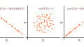
The following three plots provide a visual explanation of what it means for variables to co-vary.

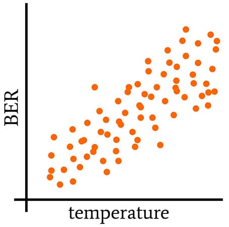
This plot represents positive covariance: when one variable increases, the other increases; when one decreases, the other decreases.

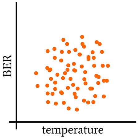
Here, an increase or a decrease in one variable can correspond to an increase or a decrease in the other variable. There’s no discernible pattern that connects one variable to the other, and the covariance is (approximately) zero.

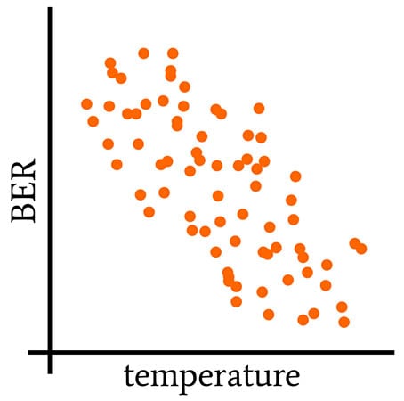
In this plot, an increase in temperature corresponds to a decrease in BER, and vice versa. Thus, the values vary together, meaning that covariance cannot be zero, but since this “togetherness” occurs in opposite directions, the covariance is negative.

Calculating Covariance

The following mathematical relationship is defined as the covariance of two variables X and Y:

\[\operatorname {cov} (X,Y)=\operatorname {E} {{\big [}(X-\operatorname {E} [X])(Y-\operatorname {E} [Y]){\big ]}}\]

For discrete data with sample size N, we have

\[\operatorname {cov} (X,Y)=\frac{1}{N-1}\sum_{i=1}^{N}(X_i-\operatorname {E}[X])(Y_i-\operatorname {E}[Y])\]

You may not be familiar with the E[X] notation. “E” stands for “expected value,” which is equal to the arithmetic mean. (There is a subtle conceptual distinction between expected value and mean, but that’s a topic for another article.) I wanted to introduce this notation because the concept of an expected value gives us another way to think about the mean of a data set—it’s the value that we expect the next measurement to be, in the sense that this expected value has the highest probability of occurrence.

The covariance formula makes intuitive sense, if you ponder it for a minute or two:

Deviations (both magnitude and polarity) in the X data set are multiplied by deviations in the Y data set.
Corresponding deviations in the two data sets that are both positive or both negative will contribute a positive quantity to the summation.
If one deviation is positive and the corresponding deviation is negative, the contribution will be negative.
When we divide the result of the summation by N—1, we are averaging all these contributions and thereby generating a value that indicates
- a tendency of the values in the two data sets to deviate in the same direction (i.e., positive covariance),
- a tendency to deviate in opposite directions (negative covariance),
- or the absence of a tendency to deviate together (zero covariance).

Conclusion

Covariance quantifies the linear correlation exhibited by two random variables. However, covariance values are somewhat difficult to interpret, and in the next article, we’ll discuss two modified versions of covariance that make correlation analysis more convenient.