Exploring Bessel Functions: Understanding the Spectrum of Tone-Modulated FM

At the end of the previous article, we learned that the spectrum of FM waves generated by a single-frequency message signal consists of an infinite number of sidebands. The sidebands are separated from each other by the modulating frequency (f_m). In practice, however, the bandwidth of an FM signal is finite. In this article, we’ll resolve this apparent contradiction and improve our overall understanding of the modulation spectrum by examining the Bessel function of the first kind.

 

Visualizing Bessel Functions

The equation for a tone-modulated FM wave with an arbitrary modulation index of β may be written as:

$$s(t) ~=~ A_c \sum_{n = - \infty}^{n = \infty} J_n(\beta) \cos \big [( \omega_c ~+~ n \omega_m)t \big ]$$

Equation 1.

 

As you can see in the equation above, the nth sideband component is scaled by J_n(β). This scaling factor is known as the Bessel function of the first kind. Figure 1 shows J_n(β) for n = 0 through 4 and β less than or equal to 20.

 

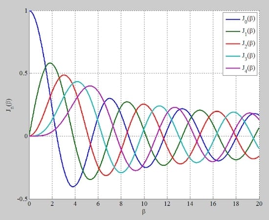
Figure 1. Bessel functions of the first kind for orders 0 through 4 and β ≤ 20.

 

When examining Figure 1, note that J₀(β) becomes zero at some values of β (2.4 and 5.5, for example). For these values of β, the carrier disappears from the output. This will be important later on in the article.

With that, let’s take a look at some of the most important properties of J_n(β).

 

The Output Spectrum When β Is Small

For small values of the modulation index (β), we can approximate J_n(β) as follows:

$$J_{n}( \beta ) ~\approx~ \frac{\beta ^ n}{2^n n!}$$

Equation 2.

 

where the symbol ! means a factorial function. When β is small enough to constitute narrowband FM, Equation 2 simplifies to:

$$\begin{cases}
J_0( \beta) ~\approx~ 1 \\
J_1( \beta) ~\approx~ \frac{\beta}{2} \\
J_n( \beta) ~\approx~ 0, \ \text{for} \ n \ge 2
\end{cases}$$

Equation 3.

 

You can visually verify these approximations by inspecting the curves in Figure 1.

For values of β much less than unity, the FM signal is composed of a carrier and a single pair of side frequencies at f_c ± f_m, similar to an AM system. For example, the magnitudes of the spectrum components for β = 0.2 are shown in Figure 2.

 

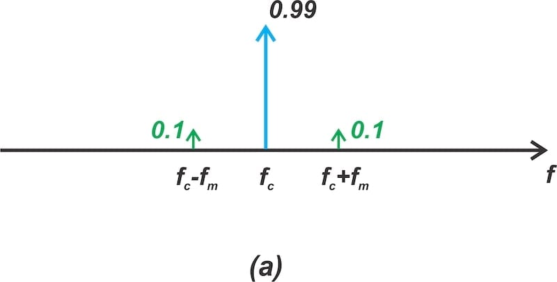
Figure 2. The magnitude of the FM signal spectrum for β = 0.2.

 

Note that the carrier component’s amplitude is close to unity and the side frequencies have an approximate amplitude of β/2 = 0.1.

 

Phase Reversal in Odd-Order Sidebands

For the Bessel function of the first kind, there’s a symmetrical relationship between the function values at positive and negative indices n. The relationship is given by:

$$J_{-n}( \beta ) ~=~ \begin{cases}
\begin{aligned}
&J_n( \beta), & n \ &\text{even} \\
&-J_n( \beta ), & n \ &\text{odd}
\end{aligned}
\end{cases}$$

Equation 4.

 

This means that the odd-order lower sidebands are phase-reversed relative to the upper sidebands of the same order. The corresponding even-order sidebands are identical.

To illustrate this, let’s once again use the example value of β = 0.2. Figure 2 showed only the magnitude of the spectrum components for this value of β. If we account for the sideband signs, we obtain the spectrum in Figure 3.

 

Figure 3. The FM signal spectrum for β = 0.2 with sideband signs taken into consideration.

 

Average Power of FM Signals

The sum of the squares of J_n(β) for all integer values of n equals unity:

$$\sum_{n=- \infty} ^{\infty} J_n^2(\beta)~=~1$$

Equation 5.

 

This property can be used to determine the average power of FM signals. Consider Equation 6, which reproduces the FM wave equation from the beginning of the article:

$$s(t) ~=~ A_c \sum_{n = - \infty}^{n = \infty} J_n(\beta) \cos \big [( \omega_c ~+~ n \omega_m)t \big ]$$

Equation 6.

 

The average power of a sum of orthogonal sinusoids is the sum of their individual powers. Hence, the average power of s(t) is:

$$P~=~ \frac{1}{2} \ A_c^2 \ \sum_{n=- \infty}^{\infty} J_n^2( \beta)$$

Equation 7.

 

Using Equation 5, the average power simplifies to:

$$P~=~ \frac{1}{2} A_c^2$$

Equation 8.

 

It’s worth mentioning that we can obtain the same result without using the identity presented in Equation 5. An angle-modulated signal may be described by:

$$s(t) ~=~ A_c \ \cos(2 \pi f_c t ~+~ \phi(t)))$$

Equation 9.

 

To compute the average power, we square the signal and take its time-average. Using a basic trigonometric identity, the square of s(t) may be written as:

$$s^2(t) ~=~ \frac{A_c^2}{2} ~+~ \frac{A_c^2}{2} \cos [2(2 \pi f_c t ~+~ \phi(t)))]$$

Equation 10.

 

Taking the time-average of this signal, we have:

$$P ~=~ \ < \Big [ \frac{A_c^2}{2} ~+~ \frac{A_c^2}{2} \cos [2(2 \pi f_c t ~+~ \phi(t)))] \Big ] > \ ~=~ \frac{A_c^2}{2}$$

Equation 11.

 

The symbol <.> in the above equation denotes the average value of the function enclosed within the brackets over time.

In finding the time-average, we note that if the carrier frequency (f_c) is large enough, the cosine term in the above equation has negligible frequency content near DC. As a result, the power in an FM wave depends on the amplitude of the unmodulated wave and is independent of the message signal. This constancy in transmitter power is a key benefit of angle modulation compared to amplitude modulation.

 

Amplitude of the Carrier Component

The amplitude of the carrier wave is scaled by the factor J₀(β). This means that the carrier wave amplitude changes with the modulation index (β), just like the sideband components. The modulation index is given by:

$$\beta ~=~ \frac{k_f A_m}{ f_m} ~=~ \frac{ \Delta f}{f_m}$$

Equation 12.

 

The carrier component is therefore dependent on the amplitude (A_m) and frequency (f_m) of the message signal, unlike in the AM scheme. As we noted in our examination of Figure 1, the carrier disappears from the output at some values of β (those at which J₀(β) equals zero).

To understand why the carrier component changes with β, recall that the average power of the FM signal is constant and equal to A_c²/2. We derived this in the previous section. In the absence of modulation, the total average power is concentrated solely in the carrier component. When the carrier undergoes frequency modulation, however, a portion of this power is distributed to the sideband components. The size of this portion is dependent on β.

The relationship between the carrier wave and the modulation index is illustrated in Figure 4 for A_c = 1.

 

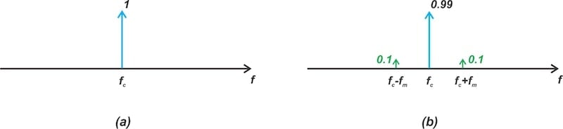
Figure 4. When β = 0, the FM signal spectrum is concentrated in the carrier component (a). Upon modulation (β = 0.2), the signal’s total power is shared between the carrier and the sideband frequencies (b).

 

Significant Sidebands of the FM Spectrum

Table 1 (which also appeared in “Introduction to Wideband FM Signals”) lists J_n(β) rounded to the nearest hundredth for selected values of β. Note that values of J_n(β) below 0.01 are deemed negligible and thus are not included in the table.

 

Table 1. Significant values of J_n(β) for n = 0 through 14 and some selected values of β.

n	Jn(0.1)	Jn(0.2)	Jn(0.5)	Jn(1)	Jn(2)	Jn(5)	Jn(10)	n
0	1.00	0.99	0.94	0.77	0.22	–0.18	–0.25	0
1	0.05	0.10	0.24	0.44	0.58	–0.33	0.04	1
2			0.03	0.11	0.35	0.05	0.25	2
3				0.02	0.13	0.36	0.06	3
4					0.03	0.39	–0.22	4
5						0.26	–0.23	5
6						0.13	–0.01	6
7						0.05	0.22	7
8						0.02	0.32	8
9							0.29	9
10							0.21	10
11							0.12	11
12							0.06	12
13							0.03	13
14							0.01	14

 

The number of significant sidebands depends on β. For instance, with β ≪ 1, only J₀(β), J₁(β), and J_-1(β) have appreciable amplitudes, implying that only the carrier and the sidebands at f_c + f_m and f_c – f_m appear at the output. As β increases, additional sidebands start to appear. Consequently, higher values of β will require a broader bandwidth for signal transmission.

When β is much greater than 1, an infinite number of sidebands will form, creating a spectrum very different from that of an amplitude modulation scheme. The data in Table 1 can be used to verify that J_n(β) exhibits a monotonic decrease for all values of n when n > β. When n is significantly greater than β, J_n(β) diminishes to well below unity.

For instance, take J_n(β) with β = 10 and varying n. When n is below 10, J_n(10) is non-monotonic. By contrast, for n > 10, it declines monotonically. This means that for a given β, J_n(β) diminishes to well below unity as n grows sufficiently. This produces only a finite number of significant sidebands.

Figure 5 demonstrates this by graphing J_n(β) against n for several values of β.

 

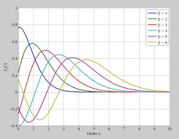
Figure 5. J_n(β) plotted as a function of n for several values of β.

 

If we assume that J_n(β) is negligible for n > β + 1, the number of significant sidebands becomes β + 1. The bandwidth of the FM wave works out to:

$$BW ~=~ 2(\beta ~+~ 1)f_m$$

Equation 13.

 

In the special case of narrowband FM, we have β ≪ 1 and the bandwidth equates to BW = 2f_m, as expected.

 

The Recurrence Relationship for J_n(β)

We’ll learn more about Equation 13 in the next article of this series. For now, I’d like to conclude by highlighting a recursive equation that relates the values of J_n(β) at different orders:

$$J_{n+1}(\beta) ~=~ \frac{2n}{\beta} J_{n}(\beta) ~-~ J_{n-1}(\beta)$$

Equation 14.

 

Using this recursive equation, we can determine J_n(β) at a specific n by knowing its values at the two preceding orders. For instance, from Table 1, we have J₀(10) = –0.25 and J₁(10) = 0.04. Substituting these values into the above equation produces:

$$\begin{eqnarray}
J_{2}(10) &~=~& \frac{2}{10} J_{1}(10) ~-~ J_{0}(10) \\
&~=~& \frac{2}{10} \times 0.04 ~-~ (-0.25) \\
&~=~& 0.258
\end{eqnarray}$$

Equation 15.

 

which, once rounding errors are taken into account, is acceptably close to the value J₂(10) = 0.25 provided in the table.

 

Wrapping Up

In order to gain a deeper understanding of the spectrum of tone-modulated FM waves, this article examined key properties of J_n(β). Our discussion highlighted the symmetry between the upper and lower sidebands, demonstrated that the total power of the FM signal remains constant, and showed that the FM signal possesses a finite effective bandwidth. We’ll discuss different ways of determining the effective bandwidth in the next article.

 

This article is Part 7 of a ten-part series on angle-modulated signals. All articles in this series are listed below in order of publication:

1. Introduction to Phase Modulation for RF Systems
2. Using Instantaneous Frequency to Represent PM and FM Signals
3. Understanding the Differences Between Phase and Frequency Modulation
4. Introduction to Narrowband Angle Modulation
5. Practical Insights Into Narrowband FM With a Single-Frequency Input
6. Introduction to Wideband FM Signals
7. Exploring Bessel Functions: Understanding the Spectrum of Tone-Modulated FM
8. Three Methods for Estimating the Transmission Bandwidth of FM Signals
9. Exploring the Relationship Between FM Wave Bandwidth and the Modulation Index
10. Estimating FM Wave Bandwidth: Solved Examples

 

All images used courtesy of Steve Arar