Understanding Noise in FM Systems: The Tone-Modulated Scenario, Part 2

This is the second half of a two-part article on how additive white Gaussian noise affects FM signals in the basic case of tone modulation, where the message is a sinusoidal signal. Part 1 used the demodulator model shown in Figure 1 and derived the output signal power.

 

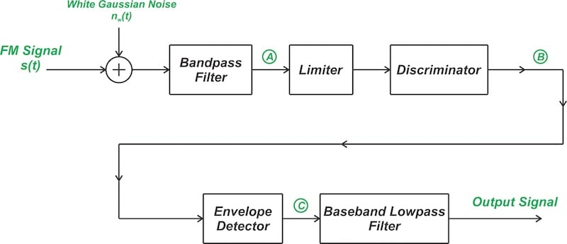
Figure 1. An FM receiver processing a noisy FM wave.

 

In this article, we trace how noise propagates through the same demodulator and derive the output noise power. We then combine the two results to find the system’s output SNR. The simplifying assumptions made across both parts will be revisited and unpacked in a follow-up article, so be sure to check it out.

 

Noise Transformation Through the Demodulator

We now present an analysis of the noise transformation as it propagates through the demodulator. Initially, the input noise n_w(t) passes through the pre-detection filter. The filtered noise n_filtered(t) at the output of the bandpass filter (node A) can be expressed in terms of its in-phase nI(t) and quadrature nQ(t) components:

$$n_{filtered}(t) = n_{I}(t) \ cos(2 \pi f_c t) - n_{Q}(t) \ sin(2 \pi f_c t)$$

Equation 1.

 

Therefore, the noisy signal applied to the limiter is:

$$s(t) + n_{filtered}(t) = A_c \cos \Big [ 2 \pi f_c t + \beta sin(2 \pi f_m t) \Big ] + n_{I}(t) \ cos(2 \pi f_c t) - n_{Q}(t) \ sin(2 \pi f_c t)$$

Equation 2.

 

To simplify noise calculations, let’s assume that there is no signal present. Put differently, the carrier wave is unmodulated (β = 0). Rearranging the terms in Equation 2, we have:

$$s(t) + n_{filtered}(t) = \Big (A_c + n_{I}(t) \Big ) \ cos(2 \pi f_c t) - n_{Q}(t) \ sin(2 \pi f_c t)$$

Equation 3.

 

This is the overall voltage at node A applied to the limiter. Using the polar representation, we rewrite Equation 3 as:

$$s(t) + n_{filtered}(t) = r_{A}(t) \ cos \big (2 \pi f_c t - \phi_{A}(t) \big )$$

Equation 4.

 

where r_A(t) and ϕ_A(t) are given by:

$$r_{A}(t) = \sqrt{ \big( A_c + n_{I}(t) \big)^2 + \big( n_{Q}(t) \big)^2} \quad and \quad \phi_{A}(t)=tan^{-1} \Big( \frac{n_{Q}(t)}{A_c + n_{I}(t)} \Big)$$

Equation 5.

 

The limiter eliminates the amplitude variations, making the multiplicative term r_A(t) irrelevant for our noise analysis. As in the signal power computation, we set the amplitude term r_A(t) to unity. We then take the time derivative of Equation 4 to determine the noise at the discriminator’s output:

$$n_{B}(t) = - \Big ( 2 \pi f_c - \frac{d \phi_{A}(t)}{dt} \Big ) \ sin \big (2 \pi f_c t - \phi_{A}(t) \big )$$

Equation 6.

 

Once we perform envelope detection and eliminate the DC term, we arrive at an expression for the noise at node C:

$$n_{C}(t) = \frac{d \phi_{A}(t)}{dt}$$

Equation 7.

 

n_C(t) is the additive noise component that appears at node C in addition to the desired message signal. Now we combine ϕ_A(t) from Equation 5 with Equation 7 to find the output noise. To simplify the calculations, we assume that the noise components n_I(t) and n_Q(t) are much smaller than the carrier amplitude A_c. Using a small argument approximation, ϕ_A(t) becomes:

$$\phi_{A}(t) \approx \frac{n_{Q}(t)}{A_c}$$

Equation 8.

 

Finally, combining Equations 7 and 8, we derive an expression for the noise at node C:

$$n_{C}(t) \approx \frac{1}{A_c} \times \frac{d }{dt}n_{Q}(t)$$

Equation 9.

 

This shows that the additive noise appearing at the output of the envelope detector depends on the carrier amplitude and the quadrature component of noise. It does not depend on the message signal. Furthermore, Equation 9 shows that the output noise is suppressed if the transmitted signal amplitude A_c is increased.

 

Calculating Average Output Noise Power

Equation 9 shows that the output noise is proportional to the time derivative of the quadrature noise component. In the frequency domain, differentiation corresponds to multiplication by jω. Therefore, the power spectral density of the noise at node C is:

$$S_{n_{C}}(\omega) = \Big | \frac{1}{A_c} \times j \omega \Big |^2 \times S_{n_{Q}}(\omega) = \frac{\omega^2}{A_c^2} \times N_0 \quad for \quad |f| \leq \frac{B_T}{2}$$

Equation 10.

 

where S_nQ(ω) denotes the power spectral density of the quadrature noise component. Note that if the white noise at the input has a two-sided spectral density of N₀/2, the in-phase and quadrature noise components will have a spectral density of N₀ around DC. This is illustrated in Figure 2 below.

 

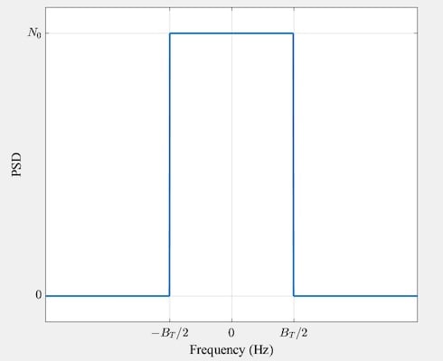
Figure 2. The power spectral density of the quadrature component.

 

Using Equation 18, the power spectral density of n_C(t) is as shown in Figure 3 below.

 

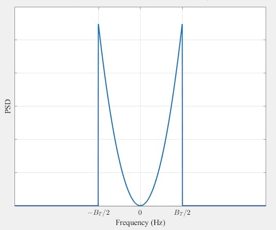
Figure 3. Power spectral density of noise at the output of the envelope detector.

 

The parabolic shape of the noise spectrum results from the differentiating action of the FM discriminator and has a profound effect on the performance of FM systems operating in the presence of noise.

If the message bandwidth is W, we usually use a lowpass filter with bandwidth W at the output. Commonly, W is smaller than B_T/2. This leads to the following noise power spectral density at the output of the lowpass filter.

$$S_{n_{o}} (\omega) = \frac{\omega^2}{A_c^2} \times N_0 \quad for \quad |f| \leq W$$

Equation 11.

 

Figure 4 shows the noise power spectral density at the output of the baseband lowpass filter for the tone-modulated case (W = f_m).

 

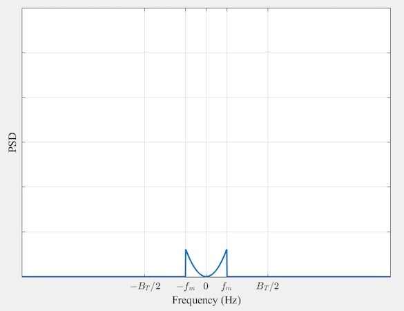
Figure 4. The power spectral density of noise at the output of the post-detection filter.

 

The average output noise power is obtained by taking the integral of the corresponding power spectral density over -ω_m to +ω_m:

$$P_{n,out} = \frac{1}{2 \pi} \int_{- \omega_m}^{+ \omega_m} S_{n_o} (\omega) \ d \omega = \frac{N_0 \omega_m^3}{3 \pi A_c^2}$$

Equation 12.

 

Note that the average output noise power is inversely proportional to the square of the carrier amplitude A_c². Therefore, increasing the carrier power has a noise-quieting effect.

This is not the case with amplitude modulation. In AM systems, the noise component is independent of the signal component. Scaling the signal power doesn’t affect the received noise power.

 

Calculating the Output SNR

The output SNR is defined as the ratio of the average output signal power to the average output noise power. Recall from Part 1 that the output signal power is Ps,out = β²ωm²/2 (Equation 8). Combining that with Equation 12, the output SNR is:

$$SNR_{out} = \frac{P_{s,out}}{P_{n, out}} = \frac{{\frac{\beta^2 \omega_m^2}{2}}}{{\frac{N_0 \omega_m^3}{3 \pi A_c^2}}} = \frac{3 \pi A_c^2\beta^2}{2N_0 \omega_m}$$

Equation 13.

 

The important point here is that the output SNR scales with the square of the modulation index β. This means that increasing β enhances the noise performance of FM systems. This relationship will be explored further in the next article.

 

Example: Determining Carrier Power for a Tone-Modulated FM Wave

Consider a tone-modulated FM wave with a message frequency of f_m = 15 kHz and modulation index of β = 5. If the noise affecting the system has a two-sided PSD of N₀/2 = 10^-14 W/Hz, what carrier power should be used to achieve an SNR of 60 dB at the output of the demodulator?

 

Solution:

Noting that the received power P_R is equal to A_c²/2, we rewrite the output SNR equation as:

$$SNR_{out} = \frac{3 \pi \beta^2}{N_0 \omega_m} \times P_R$$

Equation 14.

 

We now substitute our values into the above equation:

$$10^{6} = \frac{3 \pi \times 5^2}{2 \times 10^{-14} \times 2 \pi \times 15 \times 10^3} \times P_{R}$$

Equation 15.

 

which produces P_R = 8 microwatts. Note that a 60 dB SNR translates to a numerical value of 10⁶, which has been applied in the above calculations.

 

Wrapping Up

Together, these two articles derived the output SNR of an FM demodulator for a tone-modulated message signal. Part 1 built the demodulator model and found the output signal power. Here in Part 2, we traced how additive noise propagates through the bandpass filter, limiter, and discriminator to find the output noise power.

Combining the two results showed that the output SNR scales with the square of both the carrier amplitude and the modulation index β. This means that increasing either parameter improves the noise performance of the FM system. These articles focused on the mathematical derivation under simplifying assumptions. The next article will revisit those assumptions and visualize how signal and noise power change under FM demodulation.