Understanding Noise in FM Systems: The Tone-Modulated Scenario, Part 1

Modulation schemes vary in their response to noise because each one relies on a different signal property such as amplitude, frequency, or phase to transmit information. Since noise impacts these properties in distinct ways, we need to analyze different modulation methods to understand how they behave in the presence of noise.

This two-part article explores how additive white Gaussian noise affects FM signals, specifically in the basic case of tone modulation, where the message is a sinusoidal signal. This first part builds the demodulator model and derives the output signal power; Part 2 derives the output noise power and the resulting SNR. The simplifying assumptions made across both parts will be revisited and unpacked in a follow-up article, so be sure to check it out.

 

Preliminary Insights into FM Noise Behavior

In FM signals, the message information is encoded in the instantaneous frequency of the carrier wave. That is, in the timing of its zero crossings. Additive noise superimposed on the signal can alter the zero crossings. Figure 1 provides some insight into how FM waves with different carrier amplitudes respond to noise.

 

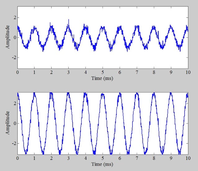
Figure 1. Impact of additive noise on FM waves with low (top) and high (bottom) carrier power.

 

The noise level is the same in both cases; however, the upper curve is generated with a smaller carrier amplitude than the lower curve. As observed, a low carrier amplitude makes zero crossings more vulnerable to noise, leading to a more corrupted FM waveform.

These example waveforms suggest that a higher carrier amplitude may offer greater immunity to noise, resulting in cleaner FM signal transmission. We’ll soon delve into the mathematical analysis to derive an expression for the FM system’s output signal-to-noise ratio (SNR). We’ll see that the mathematical analysis corroborates the intuition observed in Figure 1.

 

Methodology for Evaluating FM Noise

To aid understanding, we begin with a concise description of the noise evaluation process. Evaluating the noise performance of the FM scheme requires building a mathematical model of the system. Shown in Figure 2 is the simplified model of an FM demodulator.

 

Figure 2. Simplified FM demodulation system.

 

The core component of the system is the discriminator, which essentially extracts the phase of the incoming FM signal and outputs its time derivative. Assume the input FM wave is described by:

$$s(t)= A_c \cos \Big [ 2 \pi f_c t + \phi(t) \Big ]$$

Equation 1.

where:

A_c is the carrier amplitude

f_c is its frequency.

Then the FM demodulator produces the derivative of the phase term ϕ(t).

We use the above model to understand how the input signal and noise components change as they pass through different blocks within the FM demodulator. We then calculate the output signal-to-noise ratio to assess the quality of performance of the FM receiver.

 

More Elaborate Model of FM Demodulator

A more comprehensive representation of the FM demodulator for noise analysis is illustrated in Figure 3.

 

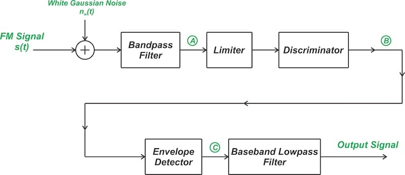
Figure 3. An FM receiver processing a noisy FM wave.

 

 

 

In the figure, s(t) is the input FM wave. It has a carrier frequency of f_c and a transmission bandwidth of B_T, which is usually determined by Carson’s rule. The transmission bandwidth B_T is approximately:

$$2(D + 1)W \text{ Hz}$$

Equation 2.

where:

W is the bandwidth of the message signal

D is the deviation ratio, which is the peak frequency deviation divided by the bandwidth W.

The noise n_w(t) denotes additive white Gaussian noise with a zero mean and a double-sided power spectral density of N₀/2 Watts/Hz.

The bandpass filter is the pre-detection filter that has a center frequency of f_c and bandwidth of B_T, enabling it to successfully pass the input FM wave without introducing any distortion. At the output of this filter (node A), we have a filtered noise process, which will be denoted by n_filtered(t) in the rest of the article.

The amplitude limiter eliminates any amplitude fluctuations in the FM wave that could result from noise or interference. By clipping the signal, it produces a rectangular wave. To eliminate the resulting harmonic distortion, the limiter employs an integral bandpass filter, which suppresses these harmonics and reconstructs the original FM wave, now free of undesired amplitude fluctuations.

The discriminator uses a slope detector that produces a hybrid-modulated wave where both amplitude and frequency vary in accordance with the message signal. The discriminator is followed by an envelope detector that generates the message signal from the amplitude variations.

Finally, the lowpass filter restricts the output bandwidth to that of the message signal, removing the out-of-band noise components, thereby minimizing the noise at the output.

We’ll now derive the SNR of the FM scheme assuming a sinusoidal message signal and applying certain simplifications. But before that, let’s have a brief overview of the FM wave equations.

 

FM Wave for Sinusoidal Message Signal

In the FM scheme, the phase term ϕ(t) is proportional to the integral of the message signal m(t), as illustrated in the equation below:

$$\phi (t) = 2 \pi k_f \int_{0}^{t} m(\tau) \ d \tau$$

Equation 3.

 

where k_f is the frequency deviation constant. For a sinusoidal message signal m(t) = A_mcos(2πf_mt), ϕ(t) is found as:

$$\phi(t) = \frac{k_f A_m}{ f_m} sin( 2 \pi f_m t)$$

Equation 4.

 

The amplitude of ϕ(t), known as the modulation index, is commonly denoted by β:

$$\beta = \frac{k_f A_m}{f_m}$$

Equation 5.

 

Therefore, with a sinusoidal message signal, the FM wave at the input of the demodulator becomes:

$$s(t)= A_c \cos \Big [ 2 \pi f_c t + \beta sin(2 \pi f_m t) \Big ]$$

Equation 6.

 

The modulation index β controls the amount of modulation in FM, playing a role analogous to the modulation index μ in conventional amplitude modulation.

 

Calculating the Output Signal Power

We seek to evaluate the output signal power resulting from the application of the FM wave described in Equation 5 to the demodulator presented in Figure 3. Since the limiter removes any amplitude variations, we infer that the signal produced at the output of the limiter has a known amplitude, which we take to be unity.

Additionally, the discriminator functions as a differentiator. Therefore, we let A_c = 1 and take the time derivative of Equation 5 to produce the discriminator output:

$$v_B(t) = \frac{d}{dt} \ s(t) = - \Big(2 \pi f_c + \beta \times 2 \pi f_m \cos(2 \pi f_m t) \Big) \times sin \Big (2 \pi f_c t+ \beta sin(2 \pi f_m t) \Big)$$

Equation 7.

 

After applying envelope detection and eliminating the constant term 2πf_c using a DC blocker, the output signal is:

$$v_o(t) = \beta \times 2 \pi f_m \ cos(2 \pi f_m t)$$

Equation 8.

 

Therefore, the output signal power is:

$$P_{s,out} = \frac{\beta^2 \omega_m^2}{2}$$

Equation 9.

 

This gives us the output signal power for the tone-modulated FM system. In Part 2, we’ll trace how additive noise propagates through the same demodulator, derive the output noise power, and combine the two results to find the system’s output SNR.