FM Generation Techniques: Solved Examples

In earlier articles of this series, we examined both direct and indirect techniques for generating FM waves. To reinforce what we learned during these discussions, this article offers four solved examples of FM modulator design. In the first two examples, we'll calculate the parameters of a reactance modulator and determine its frequency deviation. In the problems that follow, we'll explore parameter selection for an Armstrong modulator.

 

Example 1: Determining the Effective Capacitance

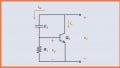
Figure 1 shows the simplified schematic of a reactance modulator.

 

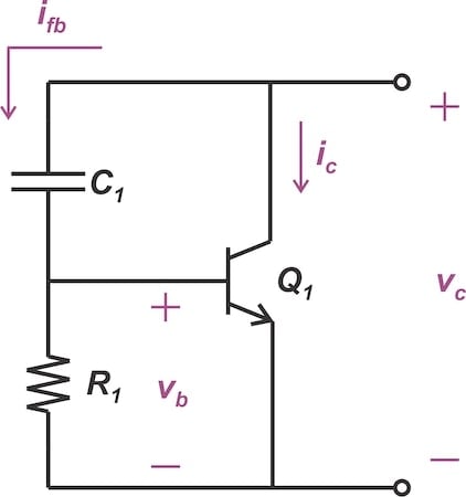
Figure 1. A basic reactance modulator.

 

The equivalent capacitance viewed from the collector-emitter terminals of this circuit is:

$$C_{eq} ~=~ g_{m} R_1 C_1$$

Equation 1.

 

where g_m is the transistor's transconductance.

Assume that at 3 MHz, the reactance of C₁ is eight times the resistance of R₁. If g_m = 12 mS, calculate the equivalent capacitance produced by the circuit.

 

Solution

Since the reactance of C₁ at the frequency of interest is eight times R₁, we have:

$$X_{C1} ~=~ \frac{1}{2 \pi f C_1} ~=~ \frac{1}{2 \pi ~\times~ 3 ~\times~ 10^6 ~\times~ C_1} ~=~ 8R_1$$

Equation 2.

 

Therefore, rearranging terms, we get:

$$R_1 C_1 ~=~ \frac{1}{2 \pi ~\times~ 24 ~\times~ 10^6}~=~6.63 ~\times~ 10^{-9}$$

Equation 3.

 

Substituting R₁C₁ from Equation 3 into Equation 1, we calculate the equivalent capacitance as:

$$C_{eq} ~=~ g_{m} R_1 C_1 ~=~ (12 ~\times~ 10^{-3}) ~\times~ (6.63 ~\times~ 10^{-9}) ~=~ 79.56 ~\times~ 10^{-12} ~=~ 79.56 \ \text{ pF}$$

Equation 4.

 

With a transconductance of g_m = 12 mS, the equivalent capacitance works out to C_eq = 79.56 pF.

 

Example 2: Determining the Frequency Deviation of the Reactance Modulator

Figure 2 shows a capacitive reactance modulator connected to the tuned circuit of an LC oscillator.

 

Figure 2. The simplified diagram of a tunable oscillator built around a reactance modulator.

 

The LC circuit has a capacitance of C₀ = 27 pF and oscillates at the carrier frequency of f_c = 88 MHz. If the message signal alters the transistor's transconductance linearly between 4 mS and 10 mS, what is the frequency deviation (Δf) of the produced FM wave? Assume that X_C1 = 10R₁ at 88 MHz.

 

Solution

Since the reactance of C₁ at f = 88 MHz is ten times greater than R₁, we have:

$$X_{C1}~=~\frac{1}{C_1 ~\times~ 2 \pi ~\times~ 88 ~\times~ 10^6} ~=~ 10R_1 \quad \Rightarrow \quad R_1 C_1 ~=~ \frac{1}{2 \pi ~\times~ 88 ~\times~ 10^7}~=~1.81 ~\times~ 10^{-10}$$

Equation 5.

 

Combining Equations 1 and 5, we now express the reactance modulator's equivalent capacitance in terms of the transconductance:

$$C_{eq} ~=~ g_m ~\times~ 1.81 ~\times~ 10^{-10}$$

Equation 6.

 

The reactance modulator produces the minimum equivalent capacitance (C_eq,min) for g_m = 4 mS:

$$C_{eq,min} ~=~ 4 ~\times~ 10^{-3} ~\times~ 1.81 ~\times~ 10^{-10} ~=~ 0.724 \ \text{pF}$$

Equation 7.

 

The maximum equivalent capacitance (C_eq,max) occurs at g_m = 10 mS:

$$C_{eq,max} ~=~ 10 ~\times~ 10^{-3} ~\times~ 1.81 ~\times~ 10^{-10} ~=~ 1.81 \ \text{pF}$$

Equation 8.

 

Therefore, the equivalent circuits at the extreme values of g_m are as shown in Figure 3.

 

Figure 3. Models of the tunable oscillator at g_m = 4 mS (left) and g_m = 10 mS (right).

 

The resonant frequency of the tank circuit, composed of the inductor (L₀) and the total capacitance (C_tot = C₀ + C_eq), can be calculated using the following formula:

$$f_r ~=~ \frac{1}{2\pi\sqrt{L_0 C_{tot}}}$$

Equation 9.

 

The lowest oscillation frequency (f_min) occurs when the total capacitance has its maximum value (C_max = C₀ + C_eq,max):

$$f_r ~=~ \frac{1}{2\pi\sqrt{L_0 C_{tot}}}$$

Equation 10.

 

Conversely, the highest oscillation frequency (f_max) occurs when the total capacitance has its minimum value (C_min = C₀ + C_eq,min):

$$f_{max} ~=~ \frac{1}{2\pi\sqrt{L_0(C_0~+~C_{eq,min})}}$$

Equation 11.

 

The ratio of the highest to the lowest oscillation frequency in our circuit is therefore given by:

$$\frac{f_{max}}{f_{min}} ~=~ \sqrt\frac{C_0 ~+~ C_{eq,max}}{C_0 ~+~ C_{eq,min}}$$

Equation 12.

 

Substituting C₀ = 27 pF, C_eq,min = 0.724 pF, and C_eq,max = 1.81 pF into the above equation, we obtain f_max/f_min = 1.019.

Finally, we note that f_max = f_c + Δf and f_min = f_c – Δf, leading to:

$$\frac{f_{c} ~+~ \Delta f}{f_{c}~-~ \Delta f} ~=~ 1.019 \quad \Rightarrow \quad 2.019 ~\times~ \Delta f ~=~ 0.019 f_c$$

Equation 13.

 

With f_c = 88 MHz, the frequency deviation works out to Δf = 828 kHz.

 

Example 3: Designing an Armstrong Modulator

Armstrong's method uses frequency multiplication to increase the frequency deviation of the FM signal. The block diagram of an Armstrong modulator is shown in Figure 4, along with the example values we'll be using in this section.

 

Figure 4. Block diagram of an Armstrong modulator with example values.

 

Suppose that the narrowband FM generator produces an FM wave with carrier frequency of f_c1 = 200 kHz and a maximum modulation index of β₁ = 0.5. The frequency of the message signal (f_m) can vary between 50 Hz and 15 kHz. If we want to produce an output FM wave with a carrier frequency of f_c4 = 96 MHz and frequency deviation of Δf₄ = 77 kHz, determine the following:

• The frequency multiplication factors (n₁ and n₂).
• The local oscillator frequency (f_LO).

 

Solution

For a tone-modulated FM wave, the modulation index (β) is given by:

$$\beta ~=~ \frac{k_f A_m}{ f_m} ~=~ \frac{ \Delta f}{f_m}$$

Equation 14.

 

where:

f_m is the frequency of the modulating signal

k_f is the frequency deviation constant

A_m is the amplitude of the modulating signal

Δf = k_fA_m is the frequency deviation.

β reaches its highest value at the lowest modulation frequency. Thus, β₁=0.5 occurs at f_m = 50 Hz, producing:

$$0.5 ~=~ \frac{ \Delta f_1}{50 \ \text{Hz}} \quad \Rightarrow \quad \Delta f_1 ~=~ 25 \ \text{Hz}$$

Equation 15.

 

Since the frequency deviation increases from Δf₁ = 25 Hz to Δf₄ = 77 kHz at the output, the total multiplication factor (n₁n₂) is:

$$n_1 n_2 ~=~ \frac{\Delta f_4}{\Delta f_1}~=~\frac{77 \ \text{kHz}}{25 \ \text{Hz}}~=~3080$$

Equation 16.

 

We now examine the carrier frequency modification along the signal path. The carrier frequency at the output of the first multiplier is f_c2 = n₁f_c1. Assuming that the mixer is used for downconversion, the carrier frequency at the output of the mixer is:

$$f_{c3} ~=~ f_{c2} ~-~ f_{LO}~=~n_1 ~\times~ f_{c1} ~-~ f_{LO}$$

Equation 17.

 

This frequency is multiplied by the second multiplier to produce the output carrier frequency:

$$f_{c4} ~=~ n_2 f_{c3} ~=~ n_1 n_{2} ~\times~ f_{c1} ~-~ n_{2} f_{LO}$$

Equation 18.

 

Noting that n₁n₂ = 3080 and substituting other parameters from the problem specification, we obtain:

$$96 \ \text{MHz} ~=~ 3080 ~\times~ 200 \ \text{kHz} ~-~ n_{2} f_{LO} \quad \Rightarrow \quad n_{2} f_{LO} ~=~ 520 \ \text{MHz}$$

Equation 19.

 

This expression does not uniquely determine n₂ and f_LO. In the absence of additional system constraints, such as the availability of a specific local oscillator, we can arbitrarily determine one parameter and calculate the other based on that choice. For example, assuming that n₂ = 48, we obtain f_LO = 10.83 MHz. Also, n₁n₂ = 3080 leads to n₁ = 64.16, which can be rounded to 64.

 

Example 4: Determining the Frequency Multiplication Factor for FM and PM Waves

Imagine a circuit that produces a narrowband angle-modulated wave with a frequency deviation of Δf₁ = 50 Hz when a 120 Hz single-tone message signal is used. The message signal has an amplitude of unity. A frequency multiplier is used after the narrowband generator to enhance the maximum frequency deviation.

Our goal is to generate a maximum frequency deviation of 20 kHz at the output of the multiplier when the message frequency applied to the narrowband generator is 240 Hz. What is the required multiplication factor if frequency modulation is used to generate the narrowband signal? What about if phase modulation (PM) is used?

 

Solution

To solve this example, we need to understand how the frequency deviations of FM and PM waves vary with the frequency of the message signal. In an FM scheme, the frequency deviation remains unaffected by the modulating frequency (f_m); in PM, it's directly proportional to f_m. This relationship, which we discussed at length in an earlier series, is illustrated in Figure 5.

 

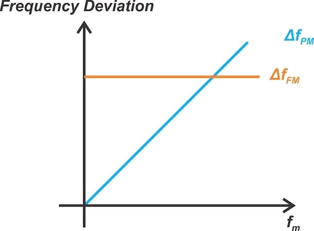
Figure 5. The impact of message frequency on the frequency deviation of FM (orange) and PM (blue) schemes.

 

First, let's assume that frequency modulation is used to generate the narrowband signal. In this case, the frequency deviation at 240 Hz is identical to that at 120 Hz, which, according to the problem specifications, is Δf₁ = 50 Hz. To increase the frequency deviation from 50 Hz to 20 kHz, we need a frequency multiplication factor of 400.

If the narrowband signal is a PM wave, then the frequency deviation is directly proportional to the message signal frequency. This means that the ratio of the frequency deviations at two different message frequencies is equal to the ratio of the frequencies. If Δf₂ is the frequency deviation at a message frequency of f_m2 = 240 Hz, we have:

$$\frac{\Delta f_2}{\Delta f_1} ~=~ \frac{f_{m2}}{f_{m1}} \quad \Rightarrow \quad \Delta f_2 ~=~ \frac{240}{120} ~\times~ 50 ~=~ 100 \ \text{Hz}$$

Equation 20.

 

In this case, a frequency multiplication factor of 200 is required to increase the frequency deviation from 100 Hz to 20 kHz.

 

Wrapping Up

Over the years, many different circuits have been developed to generate FM signals, each with its own advantages and disadvantages. In this article, we provided solved examples of FM modulator design for both the reactance modulator and Armstrong's indirect method. I hope these examples, together with the concepts presented in the previous articles, help you better appreciate the complexities in FM signal generation.

 

This article is the final installment of a seven-part series on FM signal generation. A complete list of articles in this series is provided below.

1. Introduction to Reactance Modulators for Generating FM Signals
2. An FM Generator Circuit Using the Capacitance of a Collector-Base Junction
3. Using Varactor Diodes for FM Signal Generation
4. Improving the Frequency Deviation and Stability of a Direct FM Generator
5. Understanding Varactor and PLL-Based FM Generation Using Crystal Oscillators
6. Armstrong's Method of FM Generation
7. FM Generation Techniques: Solved Examples

 

All images used courtesy of Steve Arar