Armstrong’s Method of FM Generation

FM signals can be generated using either direct or indirect methods. In the case of the former, the frequency of a voltage-controlled oscillator (VCO) is directly modulated by the message signal. Previous articles in this series covered direct FM generation at length.

Indirect FM generation takes an entirely different approach. Here, multipliers and summers are arranged to generate a narrowband signal. Frequency multiplication is then applied to increase the modulation index to the desired range of values. As a result, an indirect FM generator doesn't require the carrier oscillator to respond to a modulating signal.

The indirect method is also known as the Armstrong method or Armstrong modulator. It will be the primary focus of this article. Before we dive into this technique, however, it's essential that we understand narrowband angle-modulated signals and how they are produced.

 

Narrowband Angle-Modulated Signals

A constant-amplitude, angle-modulated signal is represented by the following equation:

$$s(t) ~=~ A_c \cos( 2 \pi f_c t ~+~ \phi(t) )$$

Equation 1.

 

Angle-modulated signals may be either phase-modulated (PM) or frequency-modulated (FM). In both cases, ϕ(t) depends on the message signal. However, the specific relationship differs depending on whether a PM or FM scheme is used. For PM, this relationship is described by Equation 2:

$$\phi (t) ~=~ k_p m(t)$$

Equation 2.

 

while for FM, we would use Equation 3:

$$\phi (t) ~=~ 2 \pi k_f \int_{0}^{t} m(\tau) \ d \tau$$

Equation 3.

 

Applying a basic trigonometric identity, we can expand Equation 1:

$$s(t) ~=~ A_c \cos( 2 \pi f_c t) cos(\phi(t) ) ~-~ A_c \sin( 2 \pi f_c t) \sin(\phi(t) )$$

Equation 4.

 

Narrowband angle modulation refers to the special case of |ϕ(t)| being much smaller than 1 radian. With |ϕ(t)| much smaller than 1 radian, we can use the following approximations:

$$\cos(\phi(t) ) ~\approx~ 1 \quad \text{and} \quad \sin(\phi(t) ) ~\approx~ \phi(t)$$

Equation 5.

 

Invoking these approximations, Equation 4 simplifies to:

$$s(t) ~\approx~ A_c \cos( 2 \pi f_c t) ~-~ A_c \phi(t) \sin(2 \pi f_c t)$$

Equation 6.

 

Note that this expression is similar to the equation for conventional AM. Any modulator for conventional AM modulation can be easily modified to generate narrowband angle-modulated signals.

 

Armstrong's Indirect Frequency Modulator

Equation 6 has an important implication for our discussion. It suggests a method for generating narrowband angle-modulated waves through the use of analog multipliers and summers. Figure 1 shows how this method is implemented.

 

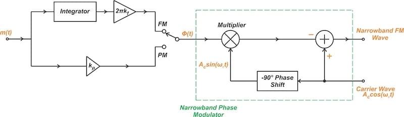
Figure 1. Generating narrowband FM signals with an integrator and narrowband phase modulator.

 

To convert the narrowband FM wave to wideband, Armstrong's method feeds the narrowband FM signal at Figure 1's output to a frequency multiplier.

Using the knowledge we've gained so far, we can construct a simplified block diagram of Armstrong's indirect FM system (Figure 2). A crystal oscillator is employed to produce a stable carrier frequency for the narrowband phase modulator.

 

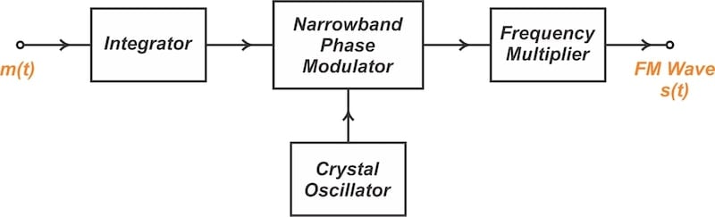
Figure 2. Simplified diagram of the indirect FM generation system.

 

To minimize the distortion from the narrowband phase modulator, it's essential to maintain a low maximum phase deviation or modulation index (β). In practice, β is typically less than 0.5.

 

Operation of the Frequency Multiplier

Figure 3 shows how a nonlinear device combined with a bandpass filter can be used to realize a frequency multiplier.

 

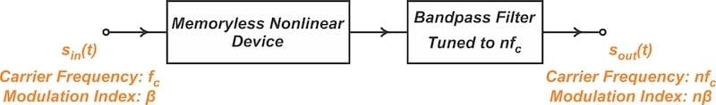
Figure 3. Block diagram of a frequency multiplier with scaling factor n.

 

To understand the operation of a frequency multiplier, consider a nonlinear device with the following input-output characteristic:

$$y(t) ~=~ a_2 x^{2}(t)$$

Equation 7.

 

where a₂ denotes the second-order nonlinearity. When an FM signal is passed through this device, the resulting output will be:

$$\begin{eqnarray}y(t) &~=~& a_2 \ \cos^2 \big ( 2 \pi f_c t ~+~ 2 \pi k_f \int_{0}^{t} m( \tau ) \ d \tau \big ) \\&~=~& \frac{a_2}{2} \bigg [ 1 ~+~ \cos \big ( 2 \pi ~\times~ 2f_c ~\times~ t ~+~ 2 ~\times~ 2 \pi k_f \int_{0}^{t} m( \tau ) \ d \tau \big ) \bigg ]\end{eqnarray}$$

Equation 8.

 

Applying this signal to a bandpass filter centered at 2f_c would eliminate the DC term. This leaves us with an FM signal that has double the input instantaneous frequency:

$$s_{out}(t) ~=~ \frac{a_2}{2} \cos \big ( 2 \pi ~\times~ 2f_c ~\times~ t ~+~ 2 ~\times~ 2 \pi k_f \int_{0}^{t} m( \tau ) \ d \tau \big )$$

Equation 9.

 

A square-law device paired with a proper bandpass filter doubles both the carrier frequency and the modulation index. An n-th law device followed by an appropriate bandpass filter will likewise increase the carrier frequency and modulation index by a factor of n. For a given message signal frequency, the peak frequency deviation (Δf) also increases by a factor of n.

In general, a memoryless nonlinear device can be described by the following characteristic:

$$y(t) ~=~ a_0 ~+~ a_1 x(t) ~+~ a_2 x^2(t) ~+~ \ldots ~+~ a_n x^n(t)$$

Equation 10.

 

It can be shown that applying an FM wave centered at f_c with a frequency deviation of Δf to Equation 10 produces output FM waves centered at f_c, 2f_c, …, nf_c with frequency deviations Δf, 2Δf, …, nΔf, respectively. Therefore, for a multiplication ratio of n, we need a device with n-th order nonlinearity. Also, the bandpass filter should be centered at nf_c and have a sufficiently large transmission bandwidth to not distort the output FM wave.

 

Limitations of Frequency Multipliers

One downside of employing frequency multipliers is the considerable loss due to harmonic generation, requiring extra amplification stages. The multiplication process also increases the phase noise at the output. Multiplying the frequency of a signal by a factor of n using an ideal frequency multiplier increases the phase noise by 20log(n) dB.

Through careful design, however, it's possible to realize multiplication factors in the range of 1,000 with just a few degrees of phase noise. Varactor and step-recovery diodes can generate high-order nonlinearities. When used as frequency multipliers, they provide multiplication factors of 10× or more in a single step.

 

The Need for Downconversion

The multiplication factor to produce the required frequency deviation is generally a large number. This means that the carrier frequency of the wideband FM would be much higher than that of the narrowband FM wave. For instance, if the carrier frequency and frequency deviation of the narrowband signal are 200 kHz and 25 Hz, respectively, and the desired frequency deviation is 75 kHz, then the frequency multiplication ratio is:

$$n ~=~ \frac{ \Delta f_{desired}}{\Delta f_{narrowband}}~=~\frac{75 \ \text{kHz}}{25 \ \text{Hz}}~=~3000$$

Equation 11.

 

To realize this large multiplication factor, several frequency doublers and triplers are cascaded. In this case, the output carrier frequency will be 200 kHz × 3000 = 600 MHz.

Such a large increase in the carrier frequency is not desirable. To reduce the carrier frequency, we can incorporate frequency mixing to shift down the carrier frequency. A mixer shifts the entire spectrum down without altering the frequency deviation of the signal. Figure 4 shows an Armstrong modulator utilizing a mixer after the frequency multiplier.

 

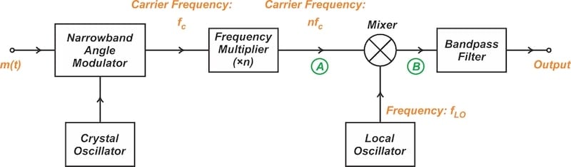
Figure 4. Indirect FM generator utilizing a mixer.

 

If the signal at the output of the frequency multiplier is:

$$s_{A}(t) ~=~ A_c \cos \Big [ 2 \pi ~\times~ nf_c ~\times~ t ~+~ n ~\times~ 2 \pi k_f \int_{0}^{t} m( \tau ) \ d \tau \Big ]$$

Equation 12.

 

and the signal produced by the local oscillator is:

$$v_{LO}(t) ~=~ 2 \cos \big ( 2 \pi ~\times~ f_{LO} ~\times~ t \big )$$

Equation 13.

 

then the signal at the output of the frequency conversion stage is:

$$\begin{eqnarray}s_{B}(t) &~=~& A_c \cos \Big [ 2 \pi (nf_c~-~f_{LO}) t ~+~ n ~\times~ 2 \pi k_f \int_{0}^{t} m( \tau ) \ d \tau \Big ] \\&~+~& A_c \cos \Big [ 2 \pi (nf_c~+~f_{LO}) t ~+~ n ~\times~ 2 \pi k_f \int_{0}^{t} m( \tau ) \ d \tau \Big ]\end{eqnarray}$$

Equation 14.

 

Employing a bandpass filter, we can keep either one of these two spectrum components and remove the other one. Assuming that a downconversion is needed, we apply a bandpass filter centered at (nf_c – f_LO), leading to:

$$s_{out}(t) ~=~ A_c \cos \Big [ 2 \pi (nf_c~-~f_{LO}) t ~+~ n ~\times~ 2 \pi k_f \int_{0}^{t} m( \tau ) \ d \tau \Big ]$$

Equation 15.

 

The frequency conversion stage is commonly a downconversion stage rather than an upconversion one. This operation requires a mixer followed by a proper bandpass filter. We can use Carson's rule to identify the bandwidth required for the bandpass filter.

 

Wrapping Up

Armstrong's method employs frequency multipliers to convert a narrowband FM signal to a wideband signal at the output. A frequency multiplier increases both the carrier frequency and the frequency deviation by the same factor.

When the output carrier frequency doesn't match the target carrier frequency, an up- or down- conversion can be employed to shift the modulated signal to the desired center frequency. While the frequency multiplier changes both the carrier frequency and deviation ratio, the mixer only changes the carrier frequency.

 

This article is Part 6 of a seven-part series on FM signal generation. All articles in this series are listed below in order of publication:

1. Introduction to Reactance Modulators for Generating FM Signals
2. An FM Generator Circuit Using the Capacitance of a Collector-Base Junction
3. Using Varactor Diodes for FM Signal Generation
4. Improving the Frequency Deviation and Stability of a Direct FM Generator
5. Understanding Varactor and PLL-Based FM Generation Using Crystal Oscillators
6. Armstrong's Method of FM Generation
7. FM Generation Techniques: Solved Examples

 

All images used courtesy of Steve Arar