Electrical Balance and Modal Analysis

In the first article of this series, we looked at how the concept of electrical balance is defined and used. We also discussed the basics of common-mode versus differential-mode signals. With our two provisional definitions (the "point" and "coupling" definitions) and our basic models to provide context, it's now time to refine our understanding by appealing to that great deity called analysis.

The examples from the previous article can be analyzed a few different ways. One particularly convenient perspective is modal analysis, which decomposes the inputs and outputs of the system into differential and common-mode components. We'll start by putting some meat on the bones of our balance discussion with mathematical modeling.

 

Introduction to Modal Analysis

In a system with two inputs and two outputs, we can view the inputs and outputs as individual excitations. Equivalently, we can define a sum and difference of the inputs (and outputs) and obtain a description of the system in these terms. In electronics, we often refer to the sum as the common mode and the difference as the differential mode.

This same concept appears everywhere in physics and engineering, though the name it's given depends on the discipline. In microwave engineering, it's called even-odd mode analysis. In control theory, they refer to the change in description as a similarity transformation. In physics, it's found as eigenmodes of a coupled mass-spring system. All of these names refer back to the same concept.

To express this idea analytically, consider Figure 1. This is a linear four-terminal network with input terminals V_i1 and V_i2 and output terminals V_o1 and V_o2.

 

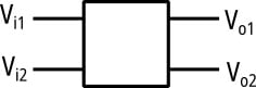
Figure 1. A four-terminal network.

 

The output terminal behavior is a function of the inputs. Assuming the system is linear, that means we can always express the outputs as a linear combination of the inputs:

$$\begin{align} V_{o 1} ~=~ a_{11}V_{i 1} ~+~ a_{12} V_{i 2} \\ V_{o 2} ~=~ a_{21}V_{i 1} ~+~ a_{22} V_{i 2} \end{align}$$

Equation 1.

 

This can be rewritten in matrix form for brevity:

$$\begin{bmatrix} V_{o1} \\ V_{o2} \end{bmatrix} ~=~ A \begin{bmatrix} V_{i 1} \\ V_{i 2} \end{bmatrix}$$

Equation 2.

 

where A is a voltage transfer function matrix.

This is a perfectly reasonable description of any linear system with two inputs and two outputs. But an equivalent representation can use Δ_i = V_i2 – V_i1 and Σ_i = V_i1 + V_i2, so that solving for V_i1 and V_i2 gives:

$$\begin{align} V_{i 1} & ~=~ \frac{\Sigma_{i}~-~\Delta_{i}}{2} \\[.5em] V_{i 2} & ~=~ \frac{\Sigma_{i} ~+~ \Delta_{i}}{2} \end{align}$$

Equation 3.

 

The transformation to Δ and Σ variables can be defined by the transformation matrix:

$$E ~=~ \begin{bmatrix} -1 & 1 \\ 1 & 1 \end{bmatrix}$$

Equation 4.

 

This is an example of a similarity transformation. It results in:

$$\begin{bmatrix} \Delta_{i} \\ \Sigma_{i} \end{bmatrix} ~=~ E \begin{bmatrix} V_{i 1} \\ V_{i 2} \end{bmatrix}$$

Equation 5.

 

and:

$$\begin{bmatrix} \Delta_{o} \\ \Sigma_{o} \end{bmatrix} ~=~ E \begin{bmatrix} V_{o 1} \\ V_{o 2} \end{bmatrix}$$

Equation 6.

 

The new output variables describe the system behavior in terms of the new input variables, according to:

$$\begin{bmatrix} \Delta_{o} \\ \Sigma_{o} \end{bmatrix} ~=~ EAE^{-1} \begin{bmatrix} \Delta_{i} \\ \Sigma_{i} \end{bmatrix}$$

Equation 7.

 

This is a transformation from one representation to another. Both are equivalent descriptions of the system. The Δ variables are differential-mode; the Σ variables are common-mode. Figure 2 shows both a traditional representation of a linear system (top) and a modal representation (bottom).

 

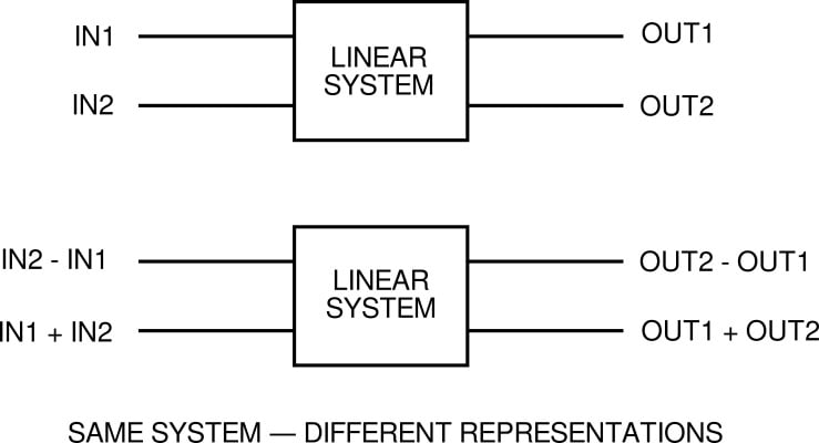
Figure 2. Transforming a linear system with two inputs and two outputs into a modal system with two input modes and two output modes.

 

Defining Common-Mode and Differential-Mode Currents

With that analysis out of the way, we can return to a simple model with a ground plane and load impedance (Figure 3).

 

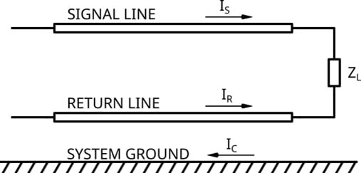
Figure 3. Two-conductor transmission line feeding a load.

 

The signal current is I_S, and the return current is I_R. Note that signal and return currents are going in the same direction.

I'll give away the plot here: we're going to define I_S and I_R in terms of common-mode and differential-mode currents. The differential-mode current is split equally between the signal and return lines. The common-mode current is split unequally between them, with a fraction (h) of the common-mode current traveling along the signal line:

$$\begin{align} & I_{S}~=~ I_{dm} ~+~ hI_{cm} \\[.5em] & I_{R} ~=~ -I_{dm} ~+~(1~-~h)I_{cm} \end{align}$$

Equation 8.

 

Deriving the Common-Mode Current

To show how we derived Equation 8, let's take the common-mode current at a position z along the transmission lines to be I_cm = I_S + I_R. In a purely differential system, I_S = –I_R, producing I_cm = 0.

In Figure 3, the current at the end of the signal line must be equal and opposite to the current at the end of the return line. The only path for the current is through the load. Therefore, there can be no common-mode current.

However, if there is any amount of capacitive coupling between the signal and return lines and system ground, then we have an alternate path for the common-mode current. Plus, if the signal and return lines are electrically long, then we can get standing current waves on the two conductors. The common-mode current is zero at the load, but non-zero elsewhere along the length of the conductors. These standing current waves tend to radiate very well.

 

Deriving the Differential-Mode Current

Above, we defined the common-mode current as I_cm = I_S + I_R. What about the differential current? Is it I_dm = I_S – I_R?

The answer is no, for both mathematical and physical reasons. First, we need to have I_S and I_R be expressible in terms of I_cm and I_dm. If I_S and I_R share the common-mode current equally, we can use:

$$\begin{align} I_{S} & ~=~ I_{dm}+\frac{I_{cm}}{2} \\ I_{R} & ~=~ -I_{dm} ~+~ \frac{I_{cm}}{2} \end{align}$$

Equation 9.

 

However, there's nothing requiring that common-mode current (the sum I_S + I_R) be shared equally between the signal and return lines. Generally, we can say that some fraction (h) of the common mode will be on the signal line, and thus a fraction equal to 1 – h will appear on the return line.

The factor h is sometimes called the current division ratio. When I_cm is equally split between the signal and return lines, then h is equal to 1/2, and we get Equation 9 for I_S and I_R. But more generally, we must use:

$$\begin{align} & I_{S}~=~ I_{dm} ~+~ hI_{cm} \\[.5em] & I_{R} ~=~ -I_{dm} ~+~(1~-~h)I_{cm} \end{align}$$

Equation 10.

 

and solving for I_dm and I_cm will give:

$$\begin{align} I_{cm} & ~=~ I_{S}+I_{R} \\ I_{dm} & ~=~ (1~-~h)I_{S} ~-~ hI_{R} \end{align}$$

Equation 11.

 

Note that while the common-mode current definition has stayed the same, the meaning of 'differential mode' is now dependent on how the common-mode current is divided between the signal and return conductors.

In some transmission lines, the value of h is constrained by physics. For example, a coax cable can only support common-mode current on the outer face of its shield (its return conductor). Therefore, we can assume h = 0 (all common-mode current is on the return conductor).

For a symmetric transmission line like twinax, twin lead, or twisted pair, there is little reason to assume the common-mode current favors one conductor over another. We can therefore take h = 1/2. Other geometries, like stripline and microstrip, are less constrained, but generally fall closer to h = 0.

 

Modal Analysis, Balance, and Mode Conversion

Using the definitions of common and differential mode above, we can restate the point definition of balance from the first article as: a two-conductor transmission line is balanced if the common-mode current equals zero. And here we can introduce another use of the word balance, to describe the way common-mode current can physically be induced on a system.

Recall that the current division factor (h) is the fraction of common-mode current which flows on the signal conductor of the transmission line. We can therefore say that the transmission line is balanced when h = 1/2. Other values of h correspond to unbalanced lines.

For example, a coax cable generally has h = 0, because the center conductor must always have current equal and opposite to the current on the inner face of the coax shield. All common-mode current must therefore flow on the outer face of the coax shield, which is uncoupled from the inner shield face and center conductor. A coax cable is therefore an unbalanced line. Conversely, a twin-lead transmission line can support common-mode current equally on both conductors, and thus it is considered a balanced transmission line.

This way of considering balance is used to great effect by Tetsushi Watanabe in his imbalance difference model, which describes the common-mode current generation at junctions between transmission lines with different current division factors. This is the mechanism behind the coax twin-lead mystery we examined in the first article.

You may recall the term mode conversion from that discussion. We can define mode conversion as the conversion of a differential-mode input into a common-mode output, or vice versa. In the coax twin-lead example, a common-mode current was excited by a differential-mode current. Figure 4 provides an illustration of this concept.

 

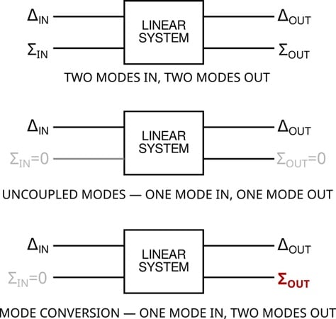
Figure 4. Mode conversion is a property of modal systems where exciting one mode causes an output in some other mode.

 

This phenomenon is worthy of our attention. Given a four-terminal network, applying a differential-mode input to the network will generally result in both differential and common-mode outputs. The relationship is usually reciprocal, so that common-mode signals induced into the system will be converted into differential-mode outputs. Unfortunately, turning common mode into differential mode threatens that desirable property, noise tolerance, of purely differential and balanced systems.

There are other sources of mode conversion, some of which we've already encountered. All of the following can be analyzed in the context of mode conversion:

• Length or phase mismatch in conductor pairs.
• Asymmetries in geometry or impedance.
• Parasitic coupling to nearby conductors.

Mode conversion can occur at a point, as with junctions between transmission lines of different h values, or it can occur in a distributed fashion along the length of the transmission line.

Modal analysis and mode conversion can be applied to domains beyond simple two-conductor transmission lines. A set of length-matched traces, a multi-conductor transmission line, even the separate windings of a wireless power transfer coil—all can be analyzed in terms of modal excitations and outputs. For this article, though, we will content ourselves with our simple models.

 

Where Do We Go From Here?

Though balance is hard to maintain, the benefits are great. The consequences of imbalance (radiation and noise coupling) can have a very negative impact on a system. The mathematical technique of modal analysis gives us a better context for analyzing balanced and unbalanced systems, but in return it demands that we carefully understand the variables being used.

These two articles have been a whirlwind of balance-related concepts. I hope you find the guidance they contain useful!

 

Featured image used courtesy of Adobe Stock; all other images used courtesy of Sam Gallagher