Facebook
 Google
 GitHub
 Linkedin
“Long’’ and “Short’’ Transmission Lines
In DC and low-frequency AC circuits, the characteristic impedance of parallel wires is usually ignored. This includes the use of coaxial cables in instrument circuits, often employed to protect weak voltage signals from being corrupted by induced “noise” caused by stray electric and magnetic fields.
This is due to the relatively short timespans in which reflections take place in the line, as compared to the period of the waveforms or pulses of the significant signals in the circuit.
As we saw in the last section, if a transmission line is connected to a DC voltage source, it will behave as a resistor equal in value to the line’s characteristic impedance only for as long as it takes the incident pulse to reach the end of the line and return as a reflected pulse, back to the source.
After that time (a brief 16.292 µs for the mile-long coaxial cable of the last example), the source “sees” only the terminating impedance, whatever that may be.
If the circuit in question handles low-frequency AC power, such short time delays introduced by a transmission line between when the AC source outputs a voltage peak and when the source “sees” that peak loaded by the terminating impedance (round-trip time for the incident wave to reach the line’s end and reflect back to the source) are of little consequence.
Even though we know that signal magnitudes along the line’s length are not equal at any given time due to signal propagation at (nearly) the speed of light, the actual phase difference between start-of-line and end-of-line signals is negligible, because line-length propagations occur within a very small fraction of the AC waveform’s period.
For all practical purposes, we can say that voltage along all respective points on a low-frequency, two-conductor line are equal and in-phase with each other at any given point in time.
In these cases, we can say that the transmission lines in question are electrically short, because their propagation effects are much quicker than the periods of the conducted signals.
By contrast, an electrically long line is one where the propagation time is a large fraction or even a multiple of the signal period. A “long” line is generally considered to be one where the source’s signal waveform completes at least a quarter-cycle (90° of “rotation”) before the incident signal reaches line’s end.
Up until this chapter in the Lessons In Electric Circuits book series, all connecting lines were assumed to be electrically short.
How to Calculate the Wavelength?
To put this into perspective, we need to express the distance traveled by a voltage or current signal along a transmission line in relation to its source frequency. An AC waveform with a frequency of 60 Hz completes one cycle in 16.66 ms.
At light speed (186,000 mile/s), this equates to a distance of 3100 miles that a voltage or current signal will propagate in that time. If the velocity factor of the transmission line is less than 1, the propagation velocity will be less than 186,000 miles per second, and the distance less by the same factor.
But even if we used the coaxial cable’s velocity factor from the last example (0.66), the distance is still a very long 2046 miles! Whatever distance we calculate for a given frequency is called the wavelength of the signal.
A simple formula for calculating wavelength is as follows:
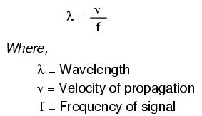
The lowercase Greek letter “lambda” (λ) represents wavelength, in whatever unit of length used in the velocity figure (if miles per second, then wavelength in miles; if meters per second, then wavelength in meters).
Velocity of propagation is usually the speed of light when calculating signal wavelength in open air or in a vacuum, but will be less if the transmission line has a velocity factor less than 1.
If a “long” line is considered to be one at least 1/4 wavelength in length, you can see why all connecting lines in the circuits discussed thus far have been assumed “short.”
For a 60 Hz AC power system, power lines would have to exceed 775 miles in length before the effects of propagation time became significant. Cables connecting an audio amplifier to speakers would have to be over 4.65 miles in length before line reflections would significantly impact a 10 kHz audio signal!
When dealing with radio-frequency systems, though, transmission line length is far from trivial. Consider a 100 MHz radio signal: its wavelength is a mere 9.8202 feet, even at the full propagation velocity of light (186,000 mile/s).
A transmission line carrying this signal would not have to be more than about 2-1/2 feet in length to be considered “long!” With a cable velocity factor of 0.66, this critical length shrinks to 1.62 feet.
What Happens if the Transmission Line is “Short”?
When an electrical source is connected to a load via a “short” transmission line, the load’s impedance dominates the circuit. This is to say, when the line is short, its own characteristic impedance is of little consequence to the circuit’s behavior.
We see this when testing a coaxial cable with an ohmmeter: the cable reads “open” from center conductor to outer conductor if the cable end is left unterminated.
Though the line acts as a resistor for a very brief period of time after the meter is connected (about 50 Ω for an RG-58/U cable), it immediately thereafter behaves as a simple “open circuit:” the impedance of the line’s open end.
Since the combined response time of an ohmmeter and the human being using it greatly exceeds the round-trip propagation time up and down the cable, it is “electrically short” for this application, and we only register the terminating (load) impedance.
It is the extreme speed of the propagated signal that makes us unable to detect the cable’s 50 Ω transient impedance with an ohmmeter.
If we use a coaxial cable to conduct a DC voltage or current to a load, and no component in the circuit is capable of measuring or responding quickly enough to “notice” a reflected wave, the cable is considered “electrically short” and its impedance is irrelevant to circuit function.
Note how the electrical “shortness” of a cable is relative to the application: in a DC circuit where voltage and current values change slowly, nearly any physical length of cable would be considered “short” from the standpoint of characteristic impedance and reflected waves.
Taking the same length of cable, though, and using it to conduct a high-frequency AC signal could result in a vastly different assessment of that cable’s “shortness!”
What Happens When the Transmission Line is Electrically “Long”?
When a source is connected to a load via a “long” transmission line, the line’s own characteristic impedance dominates over load impedance in determining circuit behavior. In other words, an electrically “long” line acts as the principal component in the circuit, its own characteristics overshadowing the load’s.
With a source connected to one end of the cable and a load to the other, current drawn from the source is a function primarily of the line and not the load. This is increasingly true the longer the transmission line is.
Consider our hypothetical 50 Ω cable of infinite length, surely the ultimate example of a “long” transmission line: no matter what kind of load we connect to one end of this line, the source (connected to the other end) will only see 50 Ω of impedance, because the line’s infinite length prevents the signal from ever reaching the end where the load is connected.
In this scenario, line impedance exclusively defines circuit behavior, rendering the load completely irrelevant.
How to Minimize the Impact of Transmission Line Length on a Circuit?
The most effective way to minimize the impact of transmission line length on circuit behavior is to match the line’s characteristic impedance to the load impedance.
If the load impedance is equal to the line impedance, then any signal source connected to the other end of the line will “see” the exact same impedance, and will have the exact same amount of current drawn from it, regardless of line length.
In this condition of perfect impedance matching, line length only affects the amount of time delay from signal departure at the source to signal arrival at the load. However, perfect matching of line and load impedances is not always practical or possible.
The next section discusses the effects of “long” transmission lines, especially when line length happens to match specific fractions or multiples of signal wavelength.
REVIEW:
- Coaxial cabling is sometimes used in DC and low-frequency AC circuits as well as in high-frequency circuits, for the excellent immunity to induced “noise” that it provides for signals.
- When the period of a transmitted voltage or current signal greatly exceeds the propagation time for a transmission line, the line is considered electrically short. Conversely, when the propagation time is a large fraction or multiple of the signal’s period, the line is considered electrically long.
- A signal’s wavelength is the physical distance it will propagate in the timespan of one period. Wavelength is calculated by the formula λ=v/f, where “λ” is the wavelength, “v” is the propagation velocity, and “f” is the signal frequency.
- A rule-of-thumb for transmission line “shortness” is that the line must be at least 1/4 wavelength before it is considered “long.”
- In a circuit with a “short” line, the terminating (load) impedance dominates circuit behavior. The source effectively sees nothing but the load’s impedance, barring any resistive losses in the transmission line.
- In a circuit with a “long” line, the line’s own characteristic impedance dominates circuit behavior. The ultimate example of this is a transmission line of infinite length: since the signal will never reach the load impedance, the source only “sees” the cable’s characteristic impedance.
- When a transmission line is terminated by a load precisely matching its impedance, there are no reflected waves and thus no problems with line length.