Facebook
 Google
 GitHub
 Linkedin
Impedance Transformation
Standing waves at the resonant frequency points of an open- or short-circuited transmission line produce unusual effects. When the signal frequency is such that exactly 1/2 wave or some multiple thereof matches the line’s length, the source “sees” the load impedance as it is.
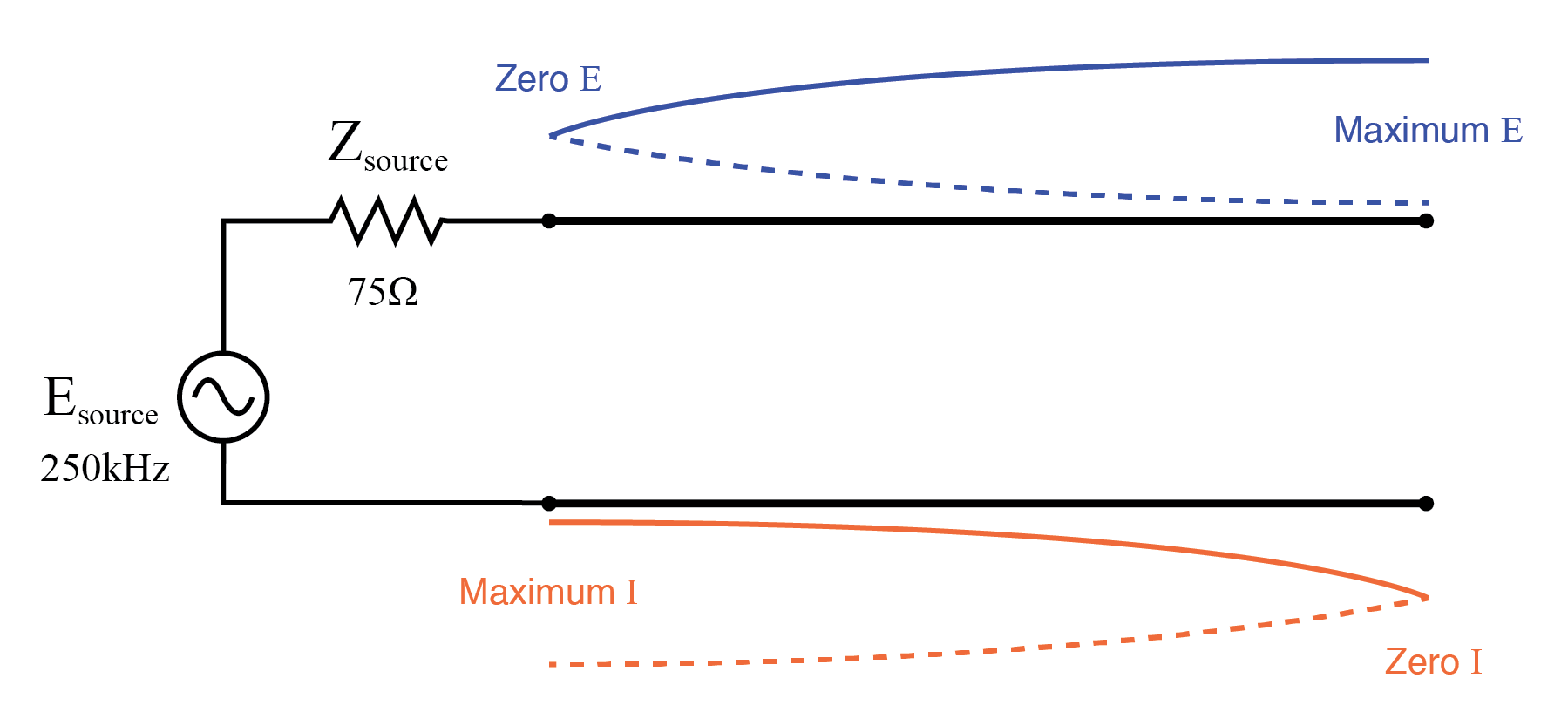
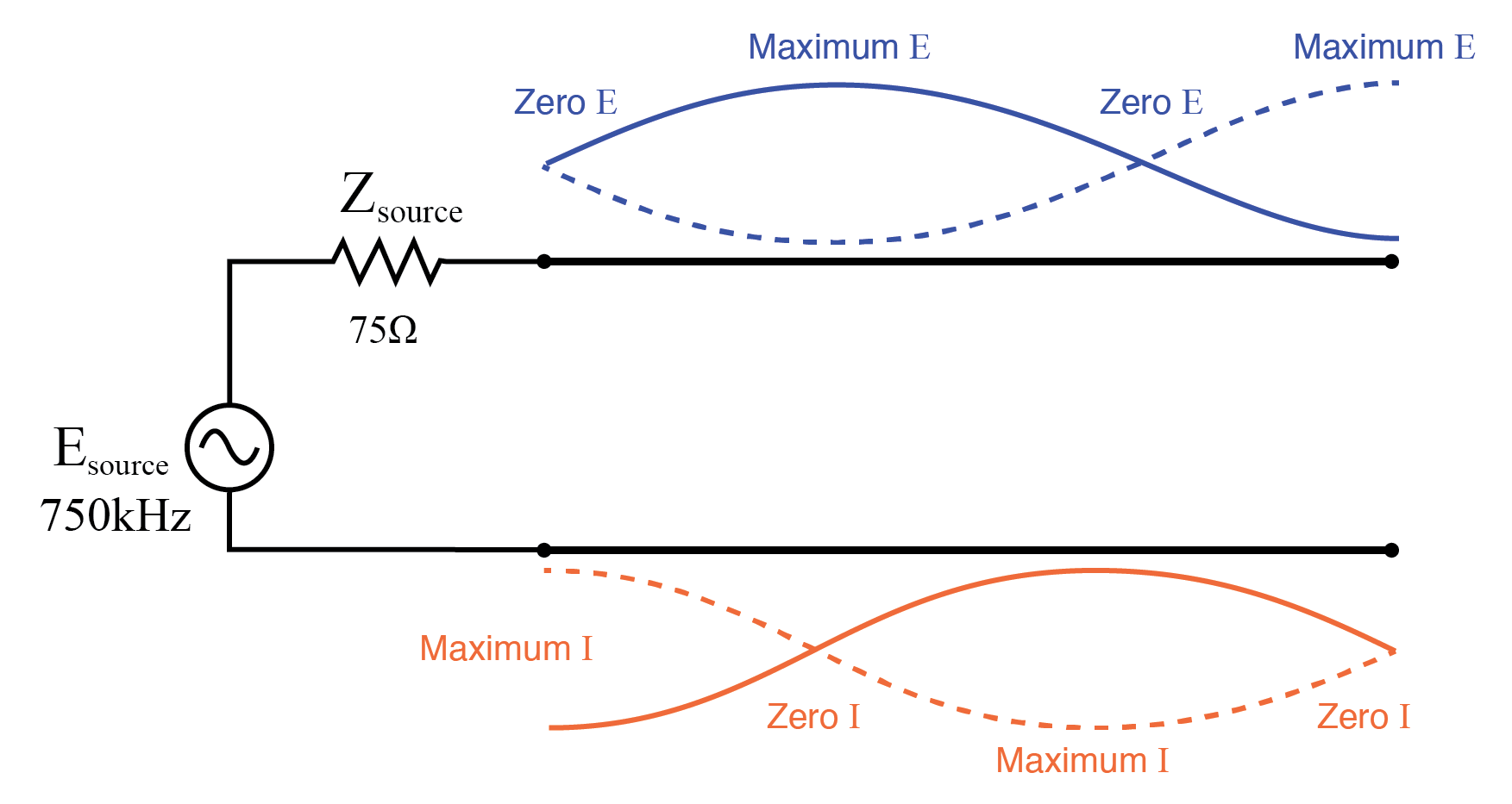
The following pair of illustrations shows an open-circuited line operating at 1/2 and 1 wavelength frequencies:
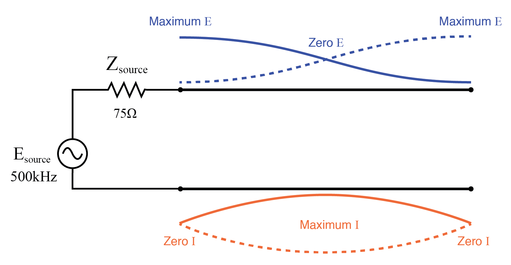
Source sees open, same as end of half wavelength line.
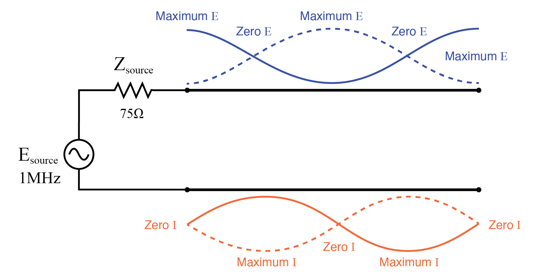
Source sees open, same as end of full wavelength (2x half wavelength line).
In either case, the line has voltage antinodes at both ends, and current nodes at both ends. That is to say, there is maximum voltage and minimum current at either end of the line, which corresponds to the condition of an open circuit.
The fact that this condition exists at both ends of the line tells us that the line faithfully reproduces its terminating impedance at the source end, so that the source “sees” an open circuit where it connects to the transmission line, just as if it were directly open-circuited.
The same is true if the transmission line is terminated by a short: at signal frequencies corresponding to 1/2 wavelength or some multiple thereof, the source “sees” a short circuit, with minimum voltage and maximum current present at the connection points between source and transmission line:
Source sees short, same as end of half wave length line.
Source sees short, same as end of full wavelength line (2x half wavelength).
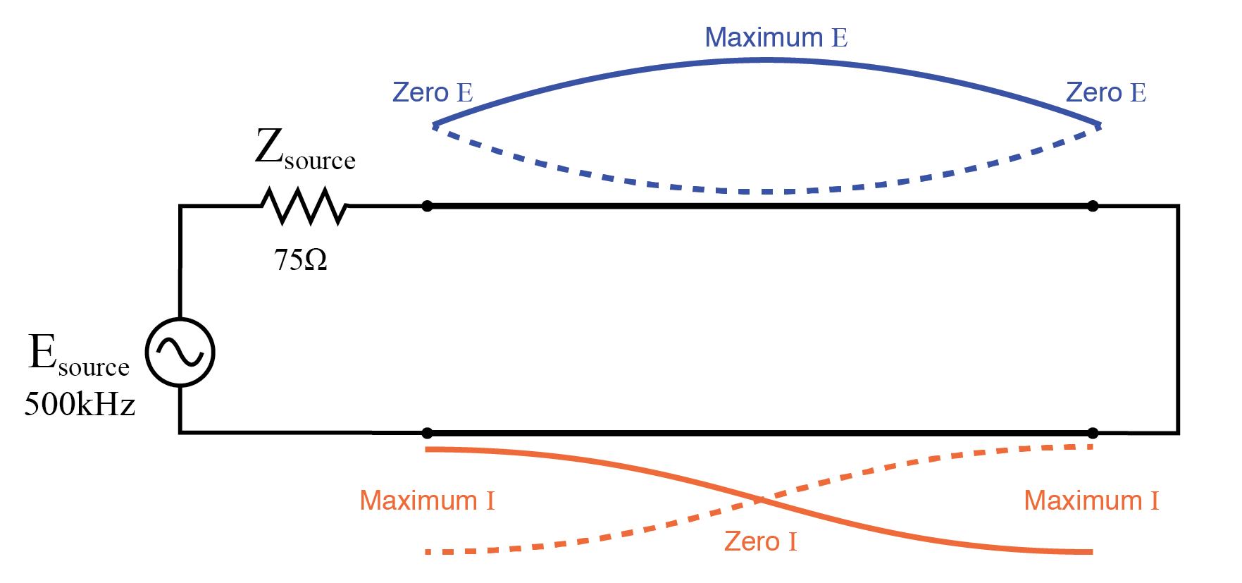
However, if the signal frequency is such that the line resonates at ¼ wavelength or some multiple thereof, the source will “see” the exact opposite of the termination impedance.
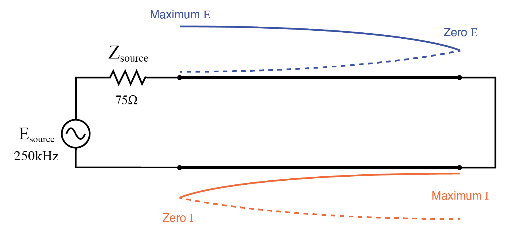
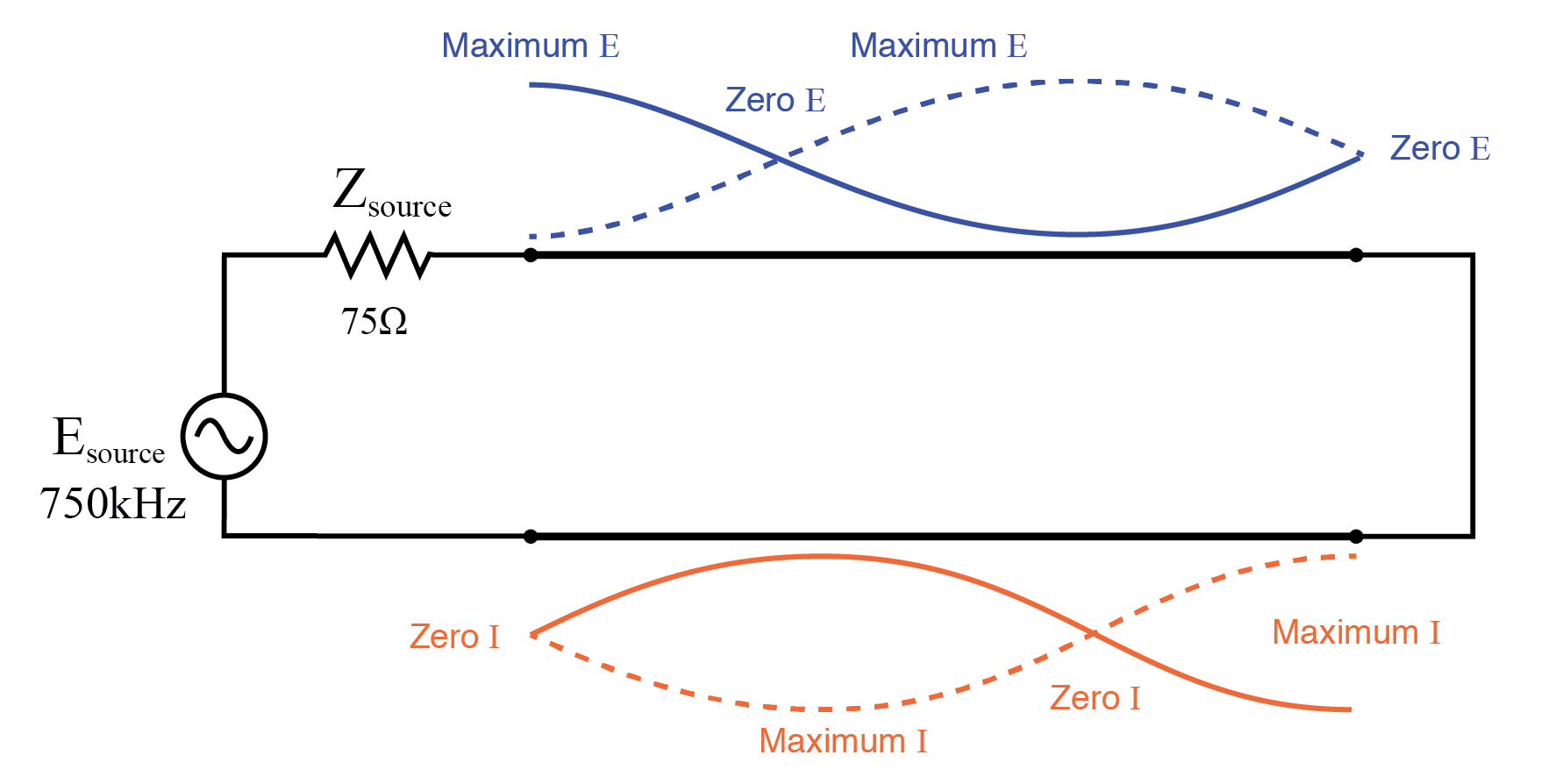
That is, if the line is open-circuited, the source will “see” a short-circuit at the point where it connects to the line; and if the line is short-circuited, the source will “see” an open circuit: (Figure below)
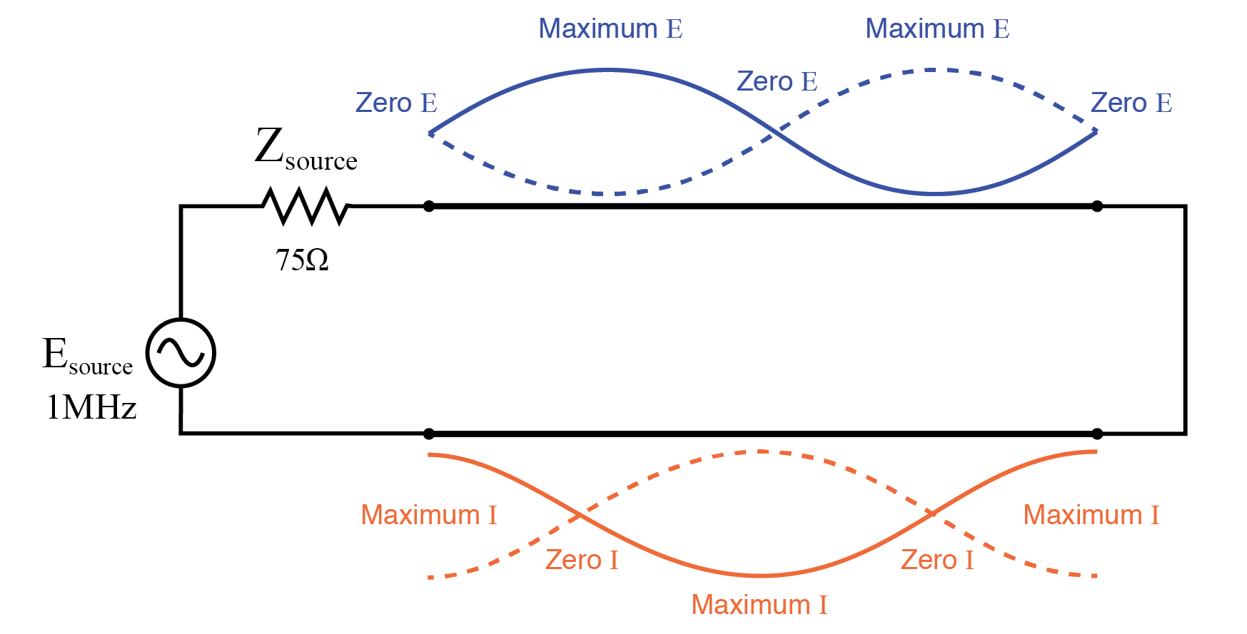
Line open-circuited; source “sees” a short circuit: at quarter wavelength line (Figure below), at three-quarter wavelength line (Figure below).
Source sees short, reflected from open at end of quarter wavelength line.
Source sees short, reflected from open at end of three-quarter wavelength line.
Line short-circuited; source “sees” an open circuit: at quarter wavelength line (Figure below), at three-quarter wavelength line (Figure below)
Source sees open, reflected from short at end of quarter wavelength line.
Source sees open, reflected from short at end of three-quarter wavelength line.
At these frequencies, the transmission line is actually functioning as an impedance transformer, transforming an infinite impedance into zero impedance, or vice versa.
Of course, this only occurs at resonant points resulting in a standing wave of 1/4 cycle (the line’s fundamental, resonant frequency) or some odd multiple (3/4, 5/4, 7/4, 9/4 . . .), but if the signal frequency is known and unchanging, this phenomenon may be used to match otherwise unmatched impedances to each other.
Take for instance the example circuit from the last section where a 75 Ω source connects to a 75 Ω transmission line, terminating in a 100 Ω load impedance.
From the numerical figures obtained via SPICE, let’s determine what impedance the source “sees” at its end of the transmission line at the line’s resonant frequencies: quarter wavelength , half wavelength, three-quarter wavelength full wavelength.
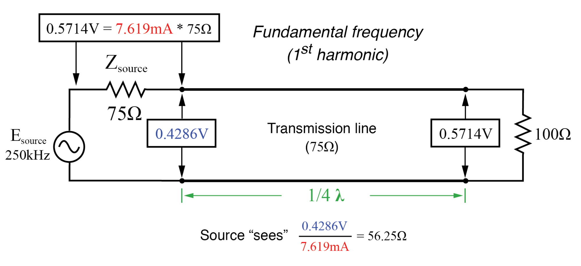
Source sees 56.25 Ω reflected from 100 Ω load at end of quarter wavelength line.
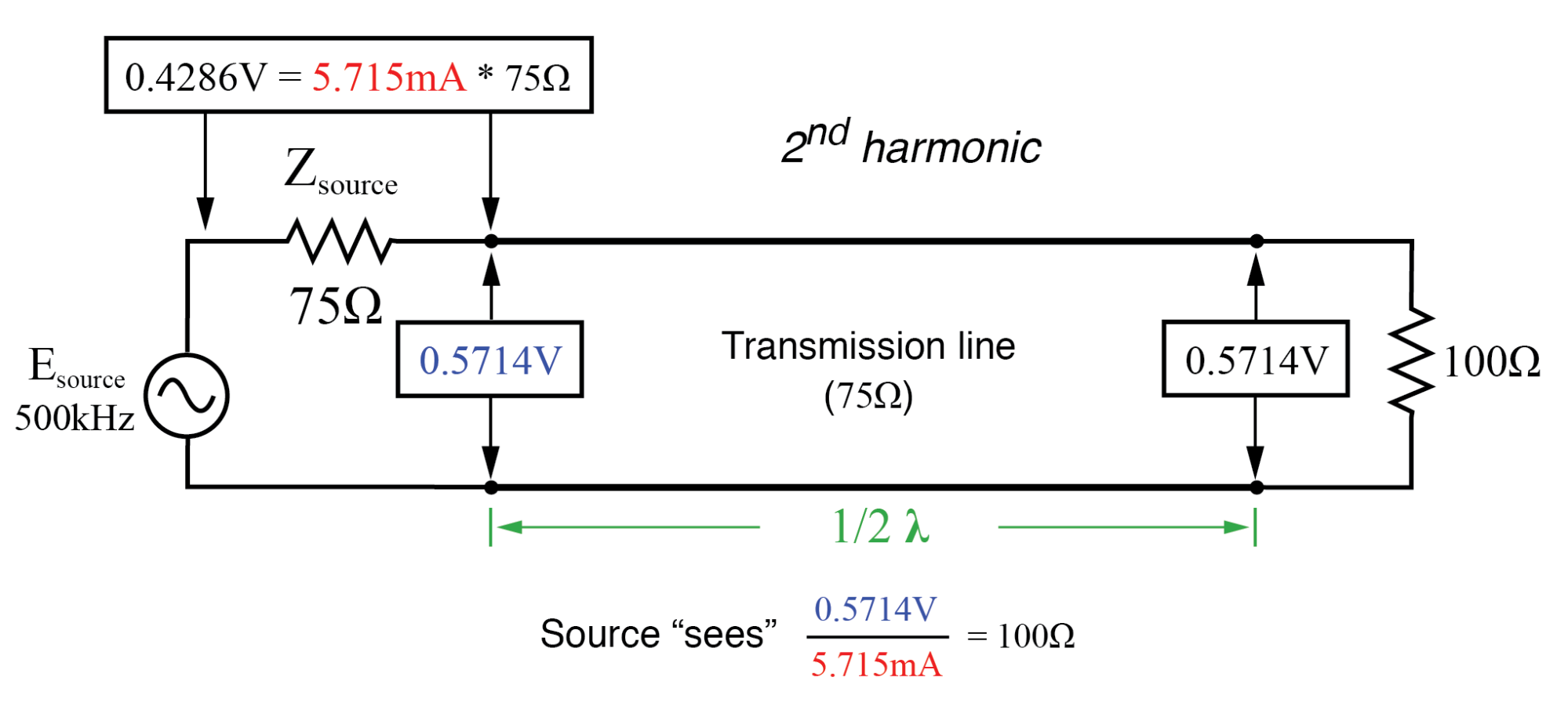
Source sees 100 Ω reflected from 100 Ω load at end of half wavelength line.
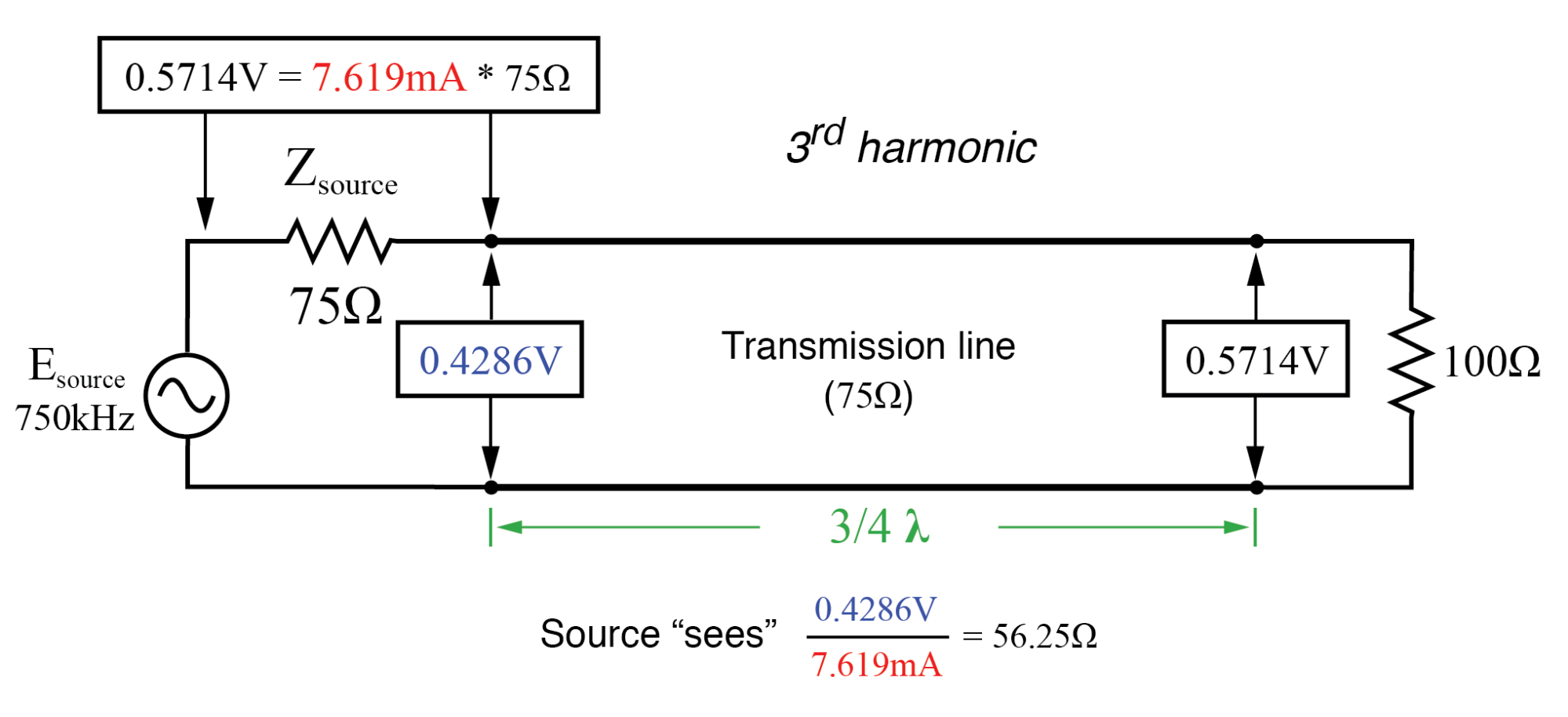
Source sees 56.25 Ω reflected from 100 Ω load at end of three-quarter wavelength line (same as quarter wavelength).
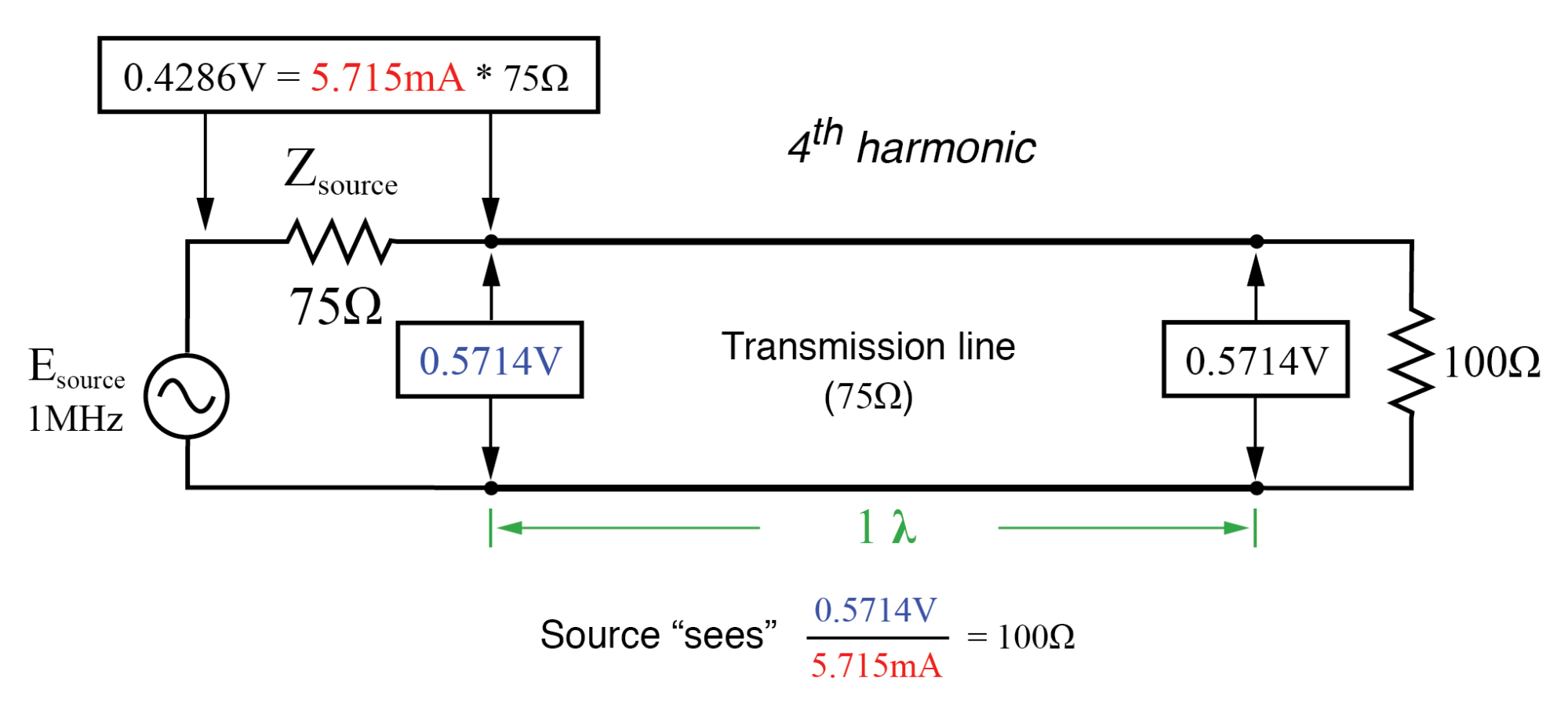
Source sees 100 Ω reflected from 100 Ω load at end of full-wavelength line (same as half-wavelength).
How Are Line, Load, and Input Impedances Related?
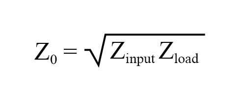
A simple equation relates line impedance (Z0), load impedance (Zload), and input impedance (Zinput) for an unmatched transmission line operating at an odd harmonic of its fundamental frequency:
One practical application of this principle would be to match a 300 Ω load to a 75 Ω signal source at a frequency of 50 MHz. All we need to do is calculate the proper transmission line impedance (Z0), and length so that exactly 1/4 of a wave will “stand” on the line at a frequency of 50 MHz.
First, calculating the line impedance: taking the 75 Ω we desire the source to “see” at the source-end of the transmission line, and multiplying by the 300 Ω load resistance, we obtain a figure of 22,500. Taking the square root of 22,500 yields 150 Ω for a characteristic line impedance.
Now, to calculate the necessary line length: assuming that our cable has a velocity factor of 0.85, and using a speed-of-light figure of 186,000 miles per second, the velocity of propagation will be 158,100 miles per second.
Taking this velocity and dividing by the signal frequency gives us a wavelength of 0.003162 miles, or 16.695 feet. Since we only need one-quarter of this length for the cable to support a quarter-wave, the requisite cable length is 4.1738 feet.
Here is a schematic diagram for the circuit, showing node numbers for the SPICE analysis we’re about to run: (Figure below)
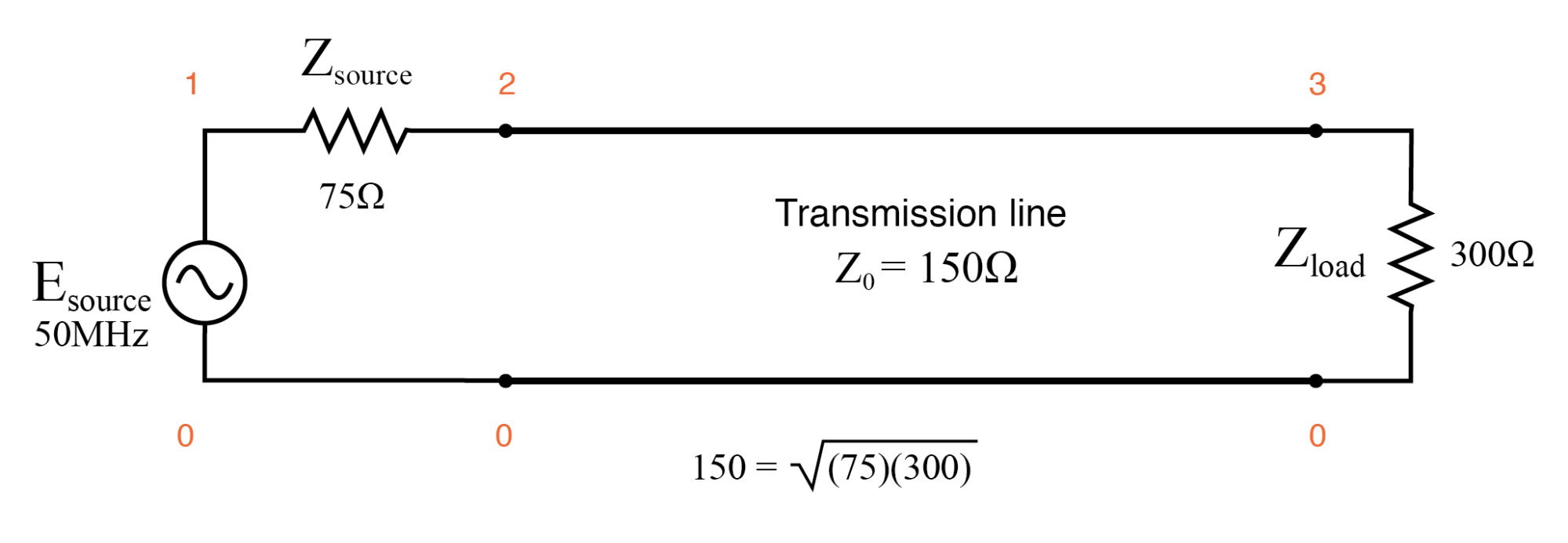
Quarter wave section of 150 Ω transmission line matches 75 Ω source to 300 Ω load.
We can specify the cable length in SPICE in terms of time delay from beginning to end. Since the frequency is 50 MHz, the signal period will be the reciprocal of that, or 20 nano-seconds (20 ns). One-quarter of that time (5 ns) will be the time delay of a transmission line one-quarter wavelength long:
Transmission line
v1 1 0 ac 1 sin
rsource 1 2 75
t1 2 0 3 0 z0=150 td=5n
rload 3 0 300
.ac lin 1 50meg 50meg
.print ac v(1,2) v(1) v(2) v(3)
.end
freq          v(1,2)      v(1)        v(2)        v(3)
5.000E+07     5.000E-01   1.000E+00   5.000E-01   1.000E+00
At a frequency of 50 MHz, our 1-volt signal source drops half of its voltage across the series 75 Ω impedance (v(1,2)) and the other half of its voltage across the input terminals of the transmission line (v(2)).
This means the source “thinks” it is powering a 75 Ω load.
The actual load impedance, however, receives a full 1 volt, as indicated by the 1.000 figure at v(3). With 0.5 volt dropped across 75 Ω, the source is dissipating 3.333 mW of power: the same as dissipated by 1 volt across the 300 Ω load, indicating a perfect match of impedance, according to the Maximum Power Transfer Theorem.
The 1/4-wavelength, 150 Ω, transmission line segment has successfully matched the 300 Ω load to the 75 Ω source.
Bear in mind, of course, that this only works for 50 MHz and its odd-numbered harmonics. For any other signal frequency to receive the same benefit of matched impedances, the 150 Ω line would have to be lengthened or shortened accordingly so that it was exactly 1/4 wavelength long.
Strangely enough, the exact same line can also match a 75 Ω load to a 300 Ω source, demonstrating how this phenomenon of impedance transformation is fundamentally different in principle from that of a conventional, two-winding transformer:
Transmission line
v1 1 0 ac 1 sin
rsource 1 2 300
t1 2 0 3 0 z0=150 td=5n
rload 3 0 75
.ac lin 1 50meg 50meg
.print ac v(1,2) v(1) v(2) v(3)
.end
freq          v(1,2)      v(1)        v(2)        v(3)
5.000E+07     5.000E-01   1.000E+00   5.000E-01   2.500E-01
Here, we see the 1-volt source voltage equally split between the 300 Ω source impedance (v(1,2)) and the line’s input (v(2)), indicating that the load “appears” as a 300 Ω impedance from the source’s perspective where it connects to the transmission line.
This 0.5 volt drop across the source’s 300 Ω internal impedance yields a power figure of 833.33 µW, the same as the 0.25 volts across the 75 Ω load, as indicated by voltage figure v(3). Once again, the impedance values of source and load have been matched by the transmission line segment.
This technique of impedance matching is often used to match the differing impedance values of transmission line and antenna in radio transmitter systems, because the transmitter’s frequency is generally well-known and unchanging.
The use of an impedance “transformer” 1/4 wavelength in length provides impedance matching using the shortest conductor length possible. (Figure below)
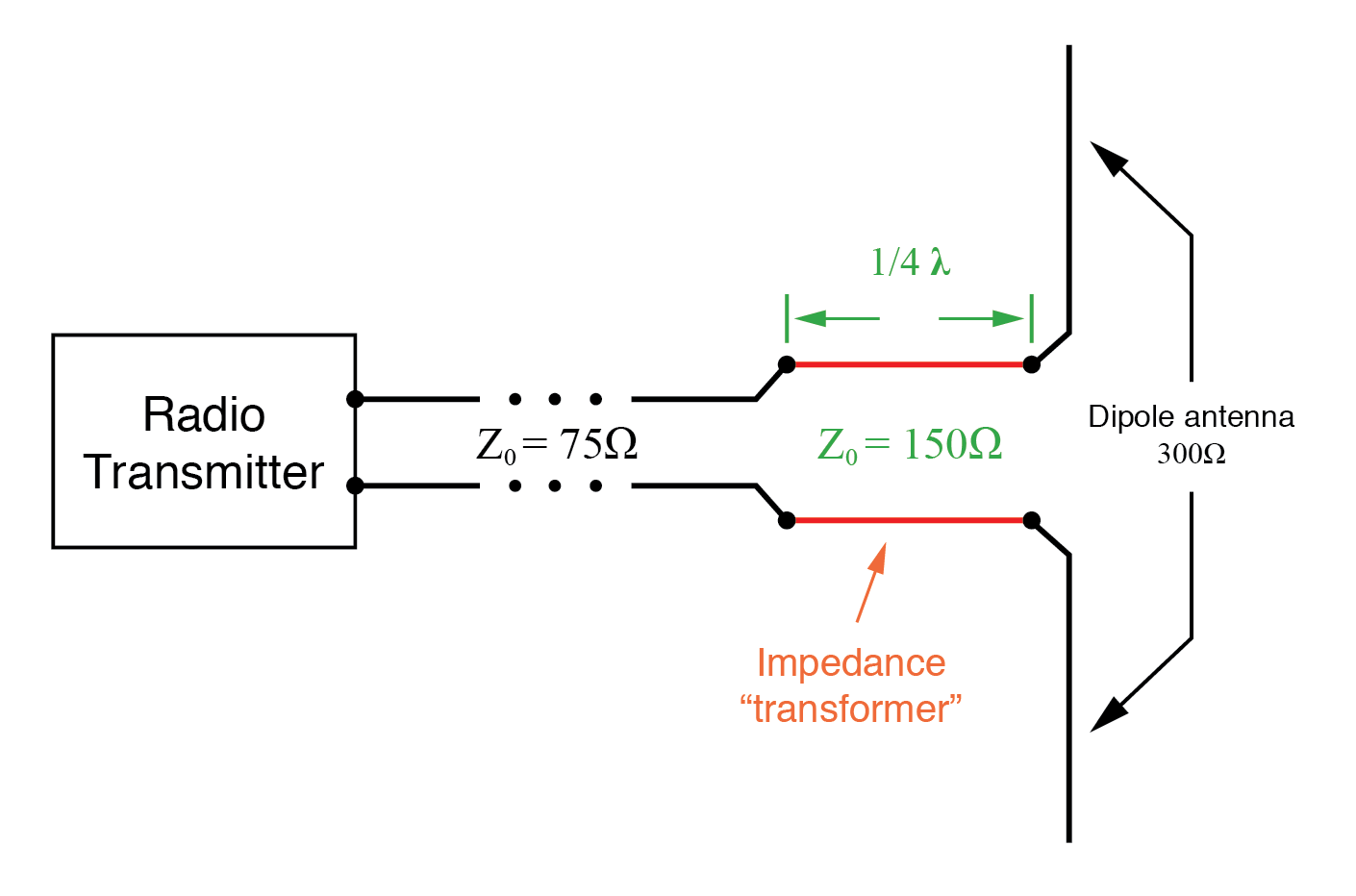
Quarter wave 150 Ω transmission line section matches 75 Ω line to 300 Ω antenna.
REVIEW:
- A transmission line with standing waves may be used to match different impedance values if operated at the correct frequency(ies).
- When operated at a frequency corresponding to a standing wave of 1/4-wavelength along the transmission line, the line’s characteristic impedance necessary for impedance transformation must be equal to the square root of the product of the source’s impedance and the load’s impedance.