Using Varactor Diodes for FM Signal Generation

In the previous article, we examined a reactance modulator that employs the collector-base junction capacitance of a BJT. The core idea of this circuit is that the collector-base junction is reverse-biased and its associated capacitance changes with the bias voltage across the junction.

Along the same lines, any semiconductor diode exhibits some capacitance variation with changes in the reverse bias voltage. In this article, we'll use a varactor diode to build a tunable oscillator for FM signal generation.

 

The Varactor-Based Modulator

Varactors are semiconductor diodes specifically designed to provide the broadest and most linear capacitance variation possible. They're also known as voltage-variable capacitors, variable-capacitance diodes, or varicaps. Figure 1 shows a varactor (C_j) connected in parallel with an LC tank circuit. The voltage source modulates the varactor bias voltage.

 

Figure 1. Using a varactor to adjust the frequency of a tuned circuit. Image used courtesy of Steve Arar

 

Note that the schematic symbol for a varactor merges the symbols of a capacitor and a diode.

Figure 2 shows how the capacitance of a typical varactor changes with the reverse bias voltage. The practical capacitance variation range for a varactor is generally limited to a specific linear section of the capacitance-voltage curve.

 

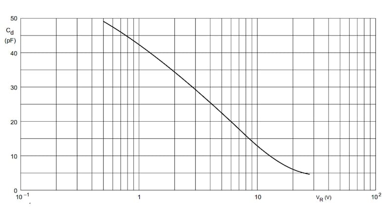
Figure 2. The BBY40 varactor's junction capacitance versus its reverse bias voltage. Image used courtesy of NXP

 

Examining Figure 2, we see that the larger the reverse voltage applied to the diode, the smaller the capacitance. The maximum capacitance of a varactor is typically in the range of 1 pF to 200 pF. The range of capacitance variation provided by a varactor can be as high as 12:1. For example, the BBY40’s capacitance can vary from about 49 pF at a bias voltage of V_D = –0.5 V to around 5 pF at V_D = –25 V, resulting in a capacitance variation range of nearly 10:1.

Figure 3 shows a typical FM generator that uses a varactor within a Colpitts-like oscillator.

 

Figure 3. An FM generator in which a varactor changes the tuned circuit of a Colpitts-like oscillator. Image used courtesy of F. Farzaneh

 

In this FM generator circuit, the control voltage (V_D) determines the DC bias voltage applied to the varactor. The audio signal from the microphone is superimposed on this DC bias, causing a shift in the varactor's capacitance. This variation in capacitance then modifies the oscillation frequency of the LC oscillator.

It should be noted that the varactor-based technique may result in a small percentage frequency deviation. To address this, we can perform frequency modulation at a higher frequency and subsequently mix the signal down to a lower frequency.

 

Determining the Frequency Deviation of the Oscillator

Let's assume that the capacitance of the resonant network consists of a fixed capacitance (C₀) shunted by a variable capacitance proportional to the message signal. The total capacitance can be represented by:

$$C_{tot} ~=~ C_0 ~+~ k_0 m(t)$$

Equation 1.

 

where k₀ is the proportionality constant and m(t) denotes the message signal. If the inductance in the resonant circuit is L₀, the output frequency for m(t) = 0 is the carrier frequency:

$$f_c ~=~ \frac{1}{2 \pi \sqrt{L_{0}C_{0}}}$$

Equation 2.

 

For non-zero m(t), however, the output frequency is obtained as:

$$f_i ~=~ \frac{1}{2 \pi \sqrt{L_{0}C_{tot}}} ~=~\frac{1}{2 \pi \sqrt{L_{0} \big ( C_0 + k_0 m(t) \big )}}$$

Equation 3.

 

This is actually the instantaneous frequency of the oscillator.

Equation 3 can be rewritten in terms of the carrier frequency (f_c) as follows:

$$f_i ~=~\frac{1}{2 \pi \sqrt{L_{0} C_{0}} \sqrt{ \big ( 1 ~+~ \frac{k_0}{C_0} m(t) \big )}}~=~ \frac{f_c}{ \sqrt{1 + \frac{k_0}{C_0} m(t)}}$$

Equation 4.

 

Assuming that |m(t)| ≤ 1 and k₀/C₀ ≪ 1, we can simplify the above expression using the following approximation:

$$\frac{1}{\sqrt{1~+~x}} \approx ~1~-~\frac{x}{2} \quad for \quad x ~\ll~1$$

Equation 5.

 

Therefore, the instantaneous frequency of the oscillator is:

$$f_i ~\approx~ f_c \big [ 1 ~-~ \frac{k_0}{2C_0} m(t) \big ] ~=~ f_c ~-~ \frac{f_c k_0}{2C_0} m(t)$$

Equation 6.

 

The second term in Equation 6 shows that m(t) linearly changes the instantaneous oscillation frequency.

Using the following equation, we can now determine the frequency deviation (|Δf|) normalized to the carrier frequency (f_c):

$$\frac{|\Delta f|}{f_c} ~\approx~ \frac{k_0}{2C_0} ~\times~ m(t)$$

Equation 7.

 

Next, we'll solidify the above concepts by looking at an example.

 

Example 1: Determining the Frequency Deviation of a Varactor-Based Modulator

Assume that the junction capacitance of a varactor can be described by:

$$C_j ~=~ \frac{C_{j0}}{\sqrt{1~-~5V_D}}$$

Equation 8.

 

where V_D is the forward bias on the junction and C_j0 is the junction capacitance for V_D = 0. This varactor is used as the capacitor of an oscillator's resonant circuit to produce direct FM signals. When the reverse bias voltage on the varactor is 4 V (or V_D = –4 V), the circuit oscillates at 10 MHz.

Now assume that we apply a small message signal m(t) riding on the DC level of –4 V to the varactor. What would be the slope of the output frequency variation relative to the input voltage?

The analysis we presented earlier assumed a linear change in varactor capacitance with the message signal (refer to Equation 1). In reality, however, the capacitance variation follows a nonlinear pattern similar to Equation 8. To use the results of our analysis, we need to linearize Equation 8 by applying the approximation from Equation 5.

The forward voltage across the varactor consists of a DC level of –4 V plus the message signal:

$$V_{D} ~=~ -4 ~+~ m(t)$$

Equation 9.

 

Substituting V_D into Equation 8, we have:

$$C_j ~=~ \frac{C_{j0}}{\sqrt{1~-~5 \big (-4 ~+~ m(t) \big) }} ~=~ \frac{C_{j0}}{\sqrt{21 ~-~ 5m(t) }}$$

Equation 10.

 

We now try to approximate C_j with a linear expression in the form of Equation 1. Applying Equation 5, we have:

$$C_j ~=~ \frac{C_{j0}}{\sqrt{21}} ~\times~ \frac{1}{ \sqrt{1 ~-~ \frac{5m(t)}{21} }} ~\approx~ \frac{C_{j0}}{\sqrt{21}} ~\times~ \big ( 1~+~ \frac{1}{2} ~\times~ \frac{5m(t)}{21} \big)$$

Equation 11.

 

Since m(t) is much less than the bias voltage of 4 V, we can assume that 5m(t)/21 is much less than unity.

Comparing Equations 1 and 11, we obtain a linearized expression for the total capacitance in the resonant circuit:

$$C_{tot} ~=~ C_0 + k_{0} m(t) \quad where \quad \begin{cases} C_0 ~=~\frac{1}{\sqrt{21}} ~\times~ C_{j0} \\ k_{0}~=~ \frac{5}{42 ~\times~\sqrt{21}} ~\times~ C_{j0} \end{cases}$$

Equation 12.

 

From Equation 6, the slope of the instantaneous frequency relative to the message signal is:

$$slope ~=~ f_c ~\times~ \frac{ k_0}{2C_0} ~=~ 10 ~\times~ 10^6 ~\times~ \frac{\frac{5}{42 ~\times~\sqrt{21}} ~\times~ C_{j0}}{2 ~\times~ \frac{1}{\sqrt{21}} ~\times~ C_{j0}} ~=~ 595.2 \ \ \text{kHz/V}$$

Equation 13.

 

Note that since the message signal is superimposed on a DC level of V_D = –4 V, the center frequency of oscillation (f_c = 10 MHz) occurs at that voltage.

To verify our calculations, we can plot the instantaneous frequency using the nonlinear capacitance equation (Equation 8). The blue curve in Figure 4 shows the actual instantaneous frequency. The green line shows the response obtained by linearizing the curve around small values of the message signal (m(t) ≈ 0).

 

Figure 4. The actual (blue) and approximated (green) instantaneous frequency versus the input signal. Image used courtesy of Steve Arar

 

The resonant circuit used in producing these curves has an inductance of L₀ = 10 µH. For a carrier frequency of 10 MHz, this means that C_j0 = 116.07 pF.

As observed, the linear response matches the actual instantaneous frequency when m(t) is small. You can use the data points shown in Figure 4 to confirm that the slope of the green line aligns with the analysis results.

 

Unsolved Example: Determining the Usable Message Signal Range

As a final exercise, determine the maximum amplitude of the message signal in the previous example. The error from the linearized curve must remain below 1% relative to the actual oscillation frequency.

Hint: To find the input range corresponding to a given error, we can substitute C_j from Equation 10 into this oscillation frequency equation:

$$f_i ~=~ \frac{1}{2 \pi \sqrt{L_{0}C_{j}}}$$

Equation 14.

 

We can then apply the binomial expansion to find the higher-order terms in the approximation.

Most of the error arises from the second-order term in the expansion. By ensuring this term remains less than 0.01 of the linear term, we can identify the input signal range that maintains an acceptably linear frequency variation at the modulator output.

 

Wrapping Up

When operated with a reverse bias, semiconductor diodes can serve as voltage-variable capacitors. The key disadvantage of the varactor-based modulator discussed in this article is that LC oscillators fail to offer a stable oscillation frequency and can drift over time due to temperature variations, supply changes, and other factors. As a result, meeting FCC requirements with LC oscillators is challenging.

To resolve this, we can use auxiliary methods for frequency stabilization. For example, as we'll explore in the next article, we can combine varactors with crystal oscillators. These deliver a precise initial oscillation frequency and superior stability over time and temperature.

 

This article is Part 3 of a seven-part series on FM signal generation. All articles in this series are listed below in order of publication:

1. Introduction to Reactance Modulators for Generating FM Signals
2. An FM Generator Circuit Using the Capacitance of a Collector-Base Junction
3. Using Varactor Diodes for FM Signal Generation
4. Improving the Frequency Deviation and Stability of a Direct FM Generator
5. Understanding Varactor and PLL-Based FM Generation Using Crystal Oscillators
6. Armstrong's Method of FM Generation
7. FM Generation Techniques: Solved Examples