Facebook
 Google
 GitHub
 Linkedin
MEMS Accelerometer Frequency Response and Bandwidth Specification
Learn about frequency response and bandwidth specification of MEMS accelerometers.
A MEMS accelerometer consists of several different mechanical and electrical components. Each of these components contributes to the overall transfer function and can limit the overall system bandwidth.
In this article, we’ll examine the frequency response of the mass-spring-damper system (sometimes written as mass-damper-spring) that plays a critical role in a MEMS accelerometer. This allows us to better understand the overall frequency response and bandwidth specification of the accelerometer.
Steady-state Response of a Mass-Spring-Damper System
In a previous article, we derived the transfer function of the mechanical part of an accelerometer as:
\[H(s) =\frac{x(s)}{a(s)} =\frac{-1}{s^2 {+\frac{b}{m}} s +\frac{k}{m}}\]
The following parameters are commonly defined to get a simpler form of the transfer function equation:
\[ \omega_n = \sqrt{ \frac{k}{m}} \]
\[ \mathcal{Q} = \frac{m \omega_n}{b}\]
where ωn and Q respectively denote the natural frequency and quality factor (also known as Q factor) of the system.
Using these parameters, we can rewrite the transfer function equation as:
\[H(s) =\frac{x(s)}{a(s)} =\frac{-1}{s^2 {+\frac{\omega_n}{\mathcal{Q}}} s +\omega^2_n}\]
Just as we use the transfer function of a circuit to predict its steady-state response to a sinusoidal input, we can use the above transfer function to determine the proof mass displacement in response to a sinusoidal acceleration at a specific frequency. For example, if the external acceleration is sinusoidal at fin given by:
\[ a(t) = \sin (2\pi \times f_{in} \times t)\]
The proof mass displacement will be:
\[ x(t) = \lvert {H(2\pi f_{in})} \lvert \space \sin(2\pi \times f_{in} \times t + \phi)\]
where |H(2πfin)| and Φ respectively denote the magnitude and phase of the transfer function at frequency fin. Note that this is the steady-state response of the system.
The system can also exhibit a transient response whenever the state of the system is changed. For example, when we first apply the sinusoidal input to a system at rest or when the sinusoidal acceleration is removed, the transient response of the system is observed. However, if we apply the sinusoidal input for a sufficiently long time, the transient response dies out and we observe the steady-state response of the system.
Magnitude of the Transfer Function
Let’s examine the derived transfer function to gain a deeper insight into the system operation. The magnitude of the transfer function is given by:
\[ \lvert {H (\omega)} \lvert = \sqrt{\frac{1}{{(\omega^2_n - \omega^2)}^2 + {(\frac{\omega_n \omega}{\mathcal{Q}})}^2}}\]
Equation 1. Finding the magnitude of the transfer function
With ωn = 2π x 500 Hz and four different Q values (0.5, 1, 1.5, 5), we obtain the curves shown below in Figure 1.
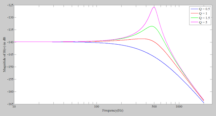
Figure 1.
As you can see, at very low frequencies, the magnitude of the transfer function is almost constant. Equation 1 gives us the value of |H(ω)| at DC (or low-frequency) acceleration as:
\[ \lvert {H (f = 0)} \lvert = \frac{1}{\omega_n} \]
As we approach the natural frequency of the system at f = 500 Hz, the magnitude of the transfer function either increases or decreases depending on the Q factor value. Above the natural frequency, the response magnitude decreases and we have a roll-off region similar to that of a low-pass electrical circuit. The mass-spring-damper system employed in a typical MEMS accelerometer exhibits gain peaking around the resonant frequency similar to the pink curve in Figure 1.
The remaining question is, at what frequency range can we use this system to measure acceleration?
The Need for a Flat Response
In order to be able to accurately measure acceleration, we need a flat response. To better understand this, assume that the external acceleration can be written as the sum of two sinusoidal terms at fin1 and fin2 as follows:
\[ a_{total} (t) = \sin (2\pi \times f_{in1} \times t) + \sin (2\pi \times f_{in2} \times t) \]
Assuming that the phase shift caused by the system is negligible, we have:
\[ x_{total} (t) = \lvert {H (2\pi f_{in1})} \lvert \thinspace \sin (2\pi \times f_{in1} \times t) + \lvert {H (2\pi f_{in2})} \lvert \thinspace \sin (2\pi \times f_{in2} \times t) \]
The total displacement will be proportional to the applied acceleration only if the system response is constant for all frequency components of interest, i.e., |H(2πfin1)| = |H(2πfin2)|. Therefore, we need a flat frequency response.
In practice, the response magnitude is not constant even at very low frequencies. Figure 2 shows a zoomed-in version of the transfer function curve for the case of ωn = 2π x 500 Hz and Q = 5.
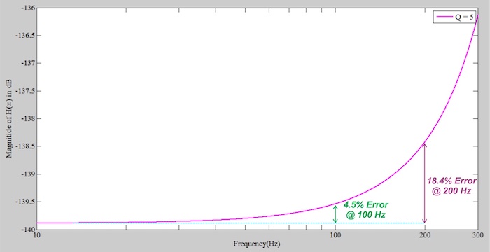
Figure 2.
You can verify that |H(f)| at 100 Hz is 4.5% higher than |H(f)| at DC (or low-frequency) acceleration. Also, |H(f)| at 200 Hz is 18.4% higher than its DC value.
The above discussion highlights an important specification of accelerometers: the accelerometer bandwidth.
Accelerometer Bandwidth Specification
The bandwidth of an accelerometer is specified as the frequency range over which the response magnitude remains within a particular maximum allowable deviation relative to the DC (or low-frequency) value of the magnitude response.
Let’s assume that the curve in Figure 2 is the overall response of an accelerometer (not just the response of the mass-spring-damper system). With the transfer function depicted in Figure 2, an effective bandwidth of 100 Hz can be considered for the system to keep the response error below 4.5%. This effective bandwidth concept might be somewhat different from the bandwidth definition used for electrical components such as amplifiers and filters. Let’s see how the bandwidth of a commercial accelerometer is defined.
The following excerpt from the ADXL1001 datasheet reveals that the 5% bandwidth of the accelerometer is 4.7 kHz.
Table 1. Frequency response information of the ADXL1001 used courtesy of Analog Devices.
| Frequency Response | |
| Sensor Resonant Frequency | 21 kHz |
| 5% Bandwidth | 4.7 kHz |
| 3 dB Bandwidth | 11 kHz |
Note that a second bandwidth specification based on the 3 dB concept is also given. This gives us the frequency at which the magnitude response changes by 3 dB compared to the DC (or low-frequency) value of the response.
The graph (Figure 3) below shows the frequency response of the ADXL1001.
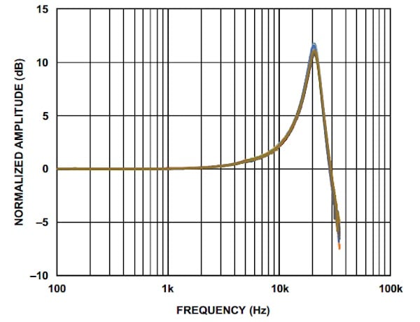
Figure 3. Image used courtesy of Analog Devices.
As you can see, the response deviation (i.e., the increase in response magnitude) originates from the gain peaking at the sensor resonant frequency.
Frequency Response of the Signal Conditioning Circuitry
In the above discussion, we only considered the frequency response of the mass-spring-damper system.
The output signal of the mass-spring-damper system is typically further processed by an internal amplifier, synchronous demodulator, and finally a low-pass filter. With some accelerometers such as the ADXL1001, the bandwidth of these electrical components is beyond the resonant frequency of the mass-spring-damper system and, hence, we observe the gain peaking around the resonant frequency in the accelerometer frequency response. However, in general, the internal low-pass filter of an accelerometer can have a cut-off frequency below the resonant frequency of the sensor and limit the overall bandwidth of the system.
In the next article, we’ll discuss how the low-pass filter limits the bandwidth and maximizes the resolution and dynamic range of the accelerometer.
To see a complete list of my articles, please visit this page.
Related Content