Facebook
 Google
 GitHub
 Linkedin
Deriving the Transfer Function of a Capacitive Sensing Accelerometer
In this article, we'll learn about deriving the transfer function of a mass-spring-damper system used in a capacitive MEMS accelerometer.
In the first part of this series, we discussed that the mass-spring-damper (or mass-damper-spring) structure can be used to measure acceleration. For the proof mass displacement to be proportional to the applied acceleration, different parameters of the mass-spring-damper system should be chosen appropriately. This article will use the concepts of classical mechanics to derive the transfer function of the mass-spring-damper system.
The transfer function allows us to describe how the proof mass moves in response to an external acceleration. The derived transfer function will be used in future articles in this series when explaining different parameters of accelerometers such as the sensor linear range of operation and bandwidth specification.
However, before attempting to derive the sensor transfer function, let’s briefly introduce the microelectromechanical systems (MEMS) technology that has enabled today’s small, low-cost inertial sensors.
MEMS Accelerometers: Measuring Acceleration With a Mass-spring-damper Structure
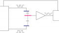
The mass-spring-damper structure used to sense acceleration is shown in Figure 1.
The MEMS technology allows us to implement a very small version of this mechanical system as well as the required signal conditioning electronics on the same silicon chip to have a complete sensing solution.
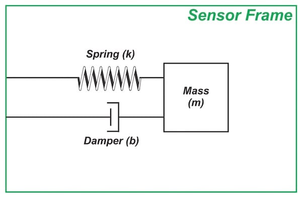
Figure 1. The mass-spring-damper structure.
MEMS technology borrows lithography-based microfabrication techniques from the microelectronics industry and combines them with additional specialized fabrication techniques that enable the creation of movable parts on a silicon chip.
The advancement in micro-fabrication technologies has helped enable today’s small, low-cost micromachined accelerometer, an example of which is shown in Figure 2.
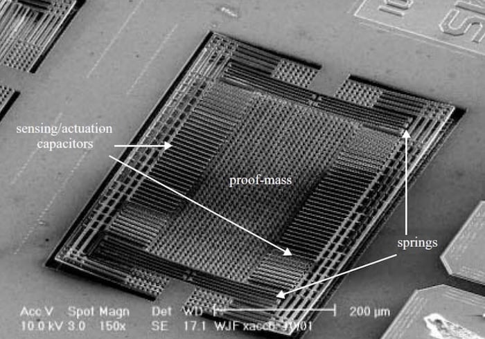
Figure 2. Scanning electron micrographs (SEM) of a CMOS MEMS accelerometer. Image used courtesy of K. Zhang
In the previous article, we briefly mentioned that a damper plays a critical role in the accelerometer operation. Now is a good time to get more familiar with this important part of the system before attempting to derive the transfer function of the mass-spring-damper system.
Damping Mechanisms in a MEMS Accelerometer
The damper models the dissipative forces that diminish the mechanical energy of the mass-spring-damper system and slow the motion of the proof mass.
One of the main damping mechanisms in MEMS accelerometers is the internal friction that occurs between the moving mass and the surrounding air molecules. In fact, it is possible to package a MEMS-based accelerometer at extremely low pressure to reduce the effect of air damping. However, in general, air damping is a major source of energy loss in a MEMS accelerometer.
Other common sources of damping are structural and thermal damping.
The structural damping takes into account the energy loss caused by the structure of the components used in MEMS devices.
The thermal damping corresponds to the deviation of the stress-strain relationship of the MEMS structures with changing temperature. The overall slowing force exerted by the damper on the proof mass is commonly modeled as a force proportional to the speed of the proof mass.
This force acts in the opposite direction of the mass motion and is given by:
\[F_{damper} = bv \]
where b denotes the damping coefficient and v denotes the speed of the proof mass.
Note that the air resistive force is proportional to an object's speed when the object is very small, which is the case for microfabricated structures.
In general, the air resistive force can have a complex relationship with an object's speed. For example, a large object, such as a skydiver moving through the air, can experience a resistive force proportional to the square of the object's speed.
Damping Effect: Desired or a Nuisance?
Since damping originates from dissipative forces, it might appear as a nuisance that should be avoided. In fact, many MEMS accelerometers are designed to have only a small amount of damping (to reduce the noise of the system).
However, it should be noted that an ideal mass-spring system with no damping is actually an oscillator and cannot be used as an accelerometer.
If we displace the mass of an "ideal" spring-mass system from equilibrium and then release it, the mass will go back and forth forever even if no external acceleration is applied to the system. This is why, for an accelerometer, we need to introduce at least a small amount of damping to our spring-mass system.
Proof Mass Displacement Using Newton’s Law of Motion
Assume that, as shown in Figure 3, an external force is applied to the sensor frame.
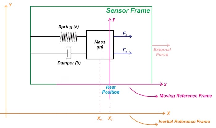
Figure 3. A mass-spring-damper structure sensor frame reacting to external force.
To calculate the proof mass displacement in terms of the applied acceleration, we use Newton’s second law of motion. As you're probably aware, this law states that the acceleration of an object as produced by a net force is directly proportional to the magnitude of the net force and inversely proportional to the mass of the object.
This is expressed by the following familiar equation:
\[F= ma \]
Equation 1
where F is the net force applied to the body, m is the mass of the body, and a denotes the acceleration.
To correctly apply this equation to our system, a subtle point should be noted here. Newton's second law of motion holds true only in inertial coordinate systems, i.e., a coordinate system that is not accelerating.
Figure 3 depicts two different coordinate systems for our accelerometer. The orange coordinate system corresponds to the Earth’s frame of reference that is assumed to be inertial when solving physics problems.
However, the magenta coordinate system represents a frame of reference fixed to the sensor frame.
This coordinate system is non-inertial because it accelerates when an external force is applied to the sensor. Therefore, to find the motion equation of the proof mass, we should use the inertial reference frame (the orange coordinate system).
What Forces Act on the Proof Mass?
Assume that, as shown in Figure 3, X0 and Xm respectively denote the rest position of the proof mass and the position of the proof mass at any particular time. With an external force in the positive X direction, the sensor frame accelerates to the right. Initially, the proof mass tends to "keep back" because of its inertia. This changes the relative position of the proof mass with respect to the sensor frame and compresses the spring by X0 – Xm. The compressed spring exerts a force on the proof mass and pushes it to the right.
The force exerted by the spring is given by:
\[F_s = k (X_0 - X_m) \]
Equation 2
As the proof mass displaces from equilibrium, the damper exerts a force proportional to the relative speed of the proof mass with respect to the rest position, we obtain:
\[F_d = b (\dot X_0 - \dot X_m) \]
Equation 3
In the above equation, the dot notation is used to show the first derivative of the variables with respect to time. As a note, the derivative of position is velocity.
Applying Equation 1, we obtain:
\[F_s + F_d = ma_{proof mass} \]
Substituting Equations 2 and 3, we arrive at
\[ k (X_0 - X_m) + b (\dot X_0 - \dot X_m) = m \ddot X_m \]
Equation 4
In this equation, the double dot notation represents the second derivative of Xm with respect to time. Note that Ẍm is the acceleration of the proof mass.
Finding the Motion Equation in the Non-Inertial Frame of Reference
It is desired to rewrite Equation 4 in terms of the proof mass displacement from its equilibrium position. This is because our sensing method in practice measures the proof mass displacement from its equilibrium.
For example, as shown in Figure 4, the capacitive sensing approach measures the proof mass displacement from a rest position.
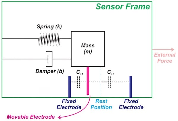
Figure 4. The setup for measuring proof mass displacement via capacitive sensing. For more information, check out the previous article in the series.
To express Equation 4 in terms of the proof mass displacement, we need to use the moving reference frame shown by the magenta coordinate system in Figure 3. We are using lowercase letters x and y for this coordinate system.
As you can see, the proof mass displacement is given by Xm – X0 = x.
In that case, Equation 4 simplifies to:
\[ -kx - b \dot x = m ( \ddot X_0 + \ddot x) \]
Since Ẍ0 is a fixed point on the sensor frame, its second derivative is equal to the acceleration of the sensor frame a. This is actually the parameter we want to measure.
Therefore, the above equation leads to:
\[ m \ddot x + b \dot x + kx = -ma \]
Finding the Transfer Function
Applying Laplace transformation, we can find the transfer function of the accelerometer as:
\[ H(s) = \frac{x(s)}{a(s)} = \frac{-1}{s^2 + \frac{b}{m}s + \frac{k}{m}} \]
This is a second-order system. Depending on the value of the system parameters, i.e., m, k, and b, the system response will be different.
For example, if the sensor frame acceleration abruptly changes from zero to a finite value (a step input), the output of the system will approach its final value with time response characteristics that are determined by the system parameters.
Figure 5 shows how changing the system parameters can change the ringing and settling time of the output. In our discussion, the output is the proof mass displacement.
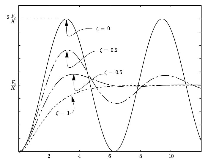
Figure 5. Step response of a second-order system can significantly change depending on the value of the system parameters. Image used courtesy of David L. Trumper via MIT
In the next article, we’ll use the derived transfer function to discuss some important system parameters such as the sensor linear range of operation, response error, and bandwidth.
To see a complete list of my articles, please visit this page.
Related Content