Facebook
 Google
 GitHub
 Linkedin
Introduction to Capacitive Accelerometers: Measuring Acceleration with Capacitive Sensing
In this article, we'll discuss how to use capacitive sensing to measure acceleration.
Accelerometers find use in different application areas. For example, in automotive applications, accelerometers are used to activate the airbag system. Cameras use accelerometers for active stabilization of pictures. Computer hard drives also rely on accelerometers to detect external shocks that can damage the read/write head of the device. In this case, the accelerometer suspends the drive operation when an external shock occurs. These are only a few accelerometer applications.
The possibilities are actually endless for what these devices can be used for. The huge advances in micro-fabrication technologies have enabled today’s small, low-cost micromachined accelerometers. In fact, the small size and low cost are two of the main factors that allow us to apply these devices to such a broad spectrum of applications.
In this article, we’ll take a look at the physics of measuring acceleration. We’ll see how a mass-spring-damper (otherwise known as a mass-damper-spring) structure can convert acceleration to a displacement quantity and how the capacitive sensing approach can be applied to convert this displacement to an electrical signal proportional to the applied acceleration.
Measuring Acceleration Using a Mass-spring-damper
A mass-spring-damper structure as shown in Figure 1 can be used to measure acceleration.
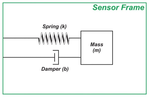
Figure 1. The mass-spring-damper structure
A known quantity of mass, commonly referred to as the proof mass (or test mass), is connected to the sensor frame through a spring.
Although the damper is a vital component of this system, we’ll shelve it until the next article in this series as it might be a bit mysterious for EEs and a few paragraphs might be required to introduce the basic concepts of a damper.
Let’s see how the structure shown in Figure 1 can detect acceleration.
When the sensor frame accelerates because of an external force, the proof mass tends to “stay back” due to its inertia. This changes the relative position of the proof mass with respect to the sensor frame as illustrated below.

Figure 2. (a) The proof mass is at its resting position when there is no external force. (b) When the frame accelerates to the right, the observer in the sensor frame observes that the proof mass is displaced to the left side of its rest position.
Figure 2(a) shows the proof mass at its resting position when there is no external force. When an external force is applied to the frame, as shown in Figure 2(b), the frame accelerates to the right. The proof mass initially tends to stay at rest, which changes the relative position of the proof mass with respect to the frame (d2 < d1).
An observer in the non-inertial (that is, accelerating) frame of the sensor observes that the proof mass is displaced to the left side of its rest position. The spring gets compressed because of the proof mass displacement and exerts a force proportional to the displacement on the proof mass. The force exerted by the spring pushes the proof mass to the right and makes it accelerate in the direction of the external force.
If appropriate values are chosen for the different parameters of the system, the proof mass displacement will be proportional to the value of the frame acceleration (after the transient response of the system dies out).
To summarize, a mass-spring-damper structure converts the acceleration of the sensor frame to the proof mass displacement. The remaining question is, how can we measure this displacement?
Measuring the Proof Mass Displacement: Capacitive Sensing Approach
The proof mass displacement can be measured by several means. One common method is the capacitive sensing approach depicted in Figure 3.
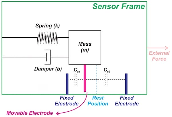
Figure 3
There are two electrodes fixed to the sensor frame along with a movable electrode connected to the proof mass. This creates two capacitors, Cs1 and Cs2, as shown in Figure 3.
As the proof mass moves in one direction, the capacitance between the movable electrode and one of the fixed electrodes increases while the capacitance of the other capacitor decreases. This is why we only need to measure the changes in the sense capacitors to detect the proof mass displacement, which is proportional to the input acceleration.
Accelerometer Signal Conditioning Using Synchronous Demodulation
To accurately measure the changes in the sense capacitors, we can apply the synchronous demodulation technique. Figure 4 shows a simplified version of the signal conditioning employed in the ADXL family of accelerometers from Analog Devices.
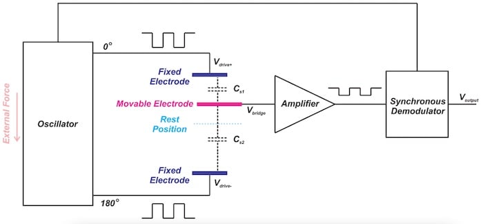
Figure 4. Image (adapted) courtesy of Analog Devices
In this case, a 1 MHz square wave is used as the AC excitation of the sense capacitors Cs1 and Cs2. The square waves applied to the fixed electrodes have the same amplitude but are 180° out of phase with respect to each other. When the movable electrode is at its resting position, the voltage at the amplifier input is zero volts.
When the movable electrode moves closer to one of the fixed electrodes, a larger portion of the excitation voltage from that electrode appears at the amplifier input Vbridge, which means the square wave that appears at the amplifier input is in-phase with the excitation voltage of the closer electrode.
For example, in Figure 4, the amplified output is a square wave in phase with Vdrive+ because Cs1 is larger than Cs2.
The amplitude of Vbridge is a function of the proof mass displacement; however, we also need to know the phase relation of Vbridge with respect to Vdrive+ and Vdrive- to determine in which direction the proof mass is displaced.
The synchronous demodulator basically multiplies the amplifier output by the excitation voltage (either Vdrive+ or Vdrive-) to convert the square wave at the amplifier output to a DC voltage that reveals the amount of displacement as well as its direction.
To learn how synchronous demodulation achieves this, please refer to my article about LVDT demodulation techniques: LVDT Demodulation: Rectifier-Type vs. Synchronous Demodulation.
Why Don’t We Use a Single Sensing Capacitor?
The capacitive sensing, depicted in Figure 3, has a differential nature: when Cs1 increases, Cs2 decreases, and vice versa.
It is also possible to employ single-ended capacitive sensing where one of the fixed electrodes is omitted, thus, there is only one variable capacitor. In this case, we can model the system as shown in Figure 5.
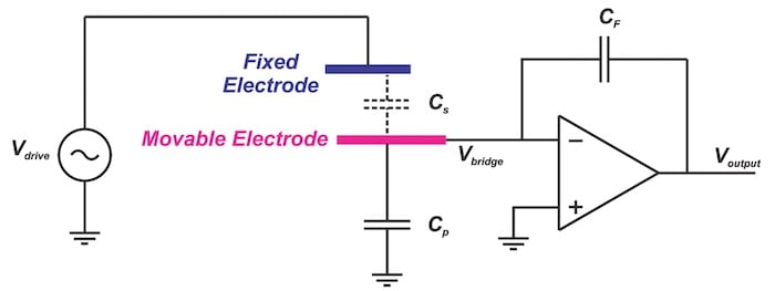
Figure 5
This single-ended version seems to be a simpler solution. So, why don’t we use a single sensing capacitor?
Single Sensing Capacitor Structure: Nonlinear Output
Let’s examine this circuit more closely.
In the above figure, Cp models the total parasitic capacitance from the movable electrode to the ground. Ideally, Vbridge is at the virtual ground and we can ignore Cp because it has ground on one side and virtual ground on the other side.
Therefore, the output can be simply obtained as:
\[ V_{output} = -\frac{C_s}{C_F} V_{drive}\]
Equation 1
Note that the bias current path is not shown in Figure 5. Using the capacitor basic equation, we can express the output in terms of the proof mass displacement.
For a capacitor C, we have:
\[ C = \epsilon \frac{A}{d}\]
Equation 2
where ε is the dielectric permittivity, A is the parallel plate area, and d is the distance between the two conductive plates. For simplicity, assume that the two capacitors Cs and CF have the same ε and A.
Equation 1 can then simplify to:
\[ V_{output} = -\frac{d_F}{d_s} V_{drive}\]
where dF and ds denote the distance between the electrodes of CF and Cs, respectively. ds can be expressed as the sum of an initial distance d0 and the displacement value Δd.
From there we can obtain:
\[ V_{output} = -\frac{d_F}{d_0 + \Delta d} V_{drive}\]
As you can see, the displacement term (Δd) is in the denominator of the output equation. Hence, the output is a nonlinear function of the proof mass displacement Δd.
Differential Structure: Linear Output
Let’s examine the transfer function of the differential capacitive sensing depicted in Figure 4.
You can verify that, with differential capacitive sensing, Vbridge is given by:
\[ V_{bridge} = \frac{C_{s1} V_{drive+} + C_{s2} V_{drive-}}{C_{s1} + C_{s2}} \]
Applying Equation 2 and assuming that the two capacitors Cs1 and Cs2 have the same ε and A values, we obtain:
\[ V_{bridge} = \frac{d_{s2} V_{drive+} + s_{s1} V_{drive-}}{d_{s1} + d_{s2}} \]
Equation 3
where ds1 and ds2 denote the distance between the electrodes of Cs1 and Cs2, respectively. When ds1 increases, ds2 decreases by the same amount and vice versa.
Assuming that:
\[ d_{s1} = d_0 - \Delta d \]
\[ d_{s2} = d_0 + \Delta d \]
\[ V_{drive+} = - V_{drive-} \]
Equation 3 simplifies to:
\[ V_{bridge} = \frac{\Delta d}{d_0} V_{drive+} \]
As you can see, with a differential structure, the output voltage is a linear function of the proof mass displacement Δd. Note that, though we could use software to remove the sensor linearity errors, having a linear response is desirable since it increases measurement precision and facilitates system calibration.
Conclusion
We saw how a mass-spring-damper structure can convert acceleration to a displacement quantity and how the capacitive sensing approach can be applied to convert this displacement to an electrical signal proportional to the applied acceleration.
We also briefly mentioned that, for the proof mass displacement to be proportional to the applied acceleration, different parameters of the mass-spring-damper system should be chosen appropriately.
In the next article, we’ll derive the transfer function of the mass-spring-damper system to gain a deeper insight into the system's operation.
To see a complete list of my articles, please visit this page.