Introduction to the Synchronous Demodulation

Sometimes, we need to measure a low-frequency signal. For example, consider a pressure sensor used in an application where the pressure changes very slowly.

The signal we are measuring is almost DC but how is this going to affect our design?

We know that at high frequencies, things can get crazy and we need to pay careful attention to every detail of the design. This might mislead us to the wrong idea that measuring a low-frequency signal is a trivial job. We’ll see that this is not necessarily the case. In fact, there is a technique called synchronous demodulation that intentionally increases the frequency of operation to achieve a more accurate measurement.

This article will discuss the basic idea behind the synchronous demodulation technique. 

 

Example of Low-Frequency Measurement

There are applications where a sensor with a low-frequency output is measured directly (without applying synchronous demodulation). For example, the electret microphone is a special type of variable capacitance that is measured directly. The capacitance of an electret microphone varies with air pressure variations (sound waves).

A Teflon-like material, called electret, that has a fixed charge bonded to its surface is used in the capacitor structure. Since the charge on the capacitor is fixed, the change in the capacitance value caused by the air pressure variations leads to a corresponding change in the voltage across the capacitor (For a capacitor, we have Q=CV).

As shown in Figure 1, an electret microphone usually has an internal JFET that acts as a buffer.

 

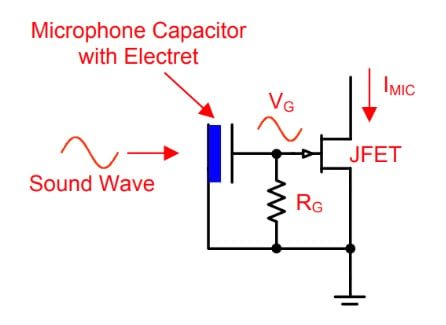
Figure 1. Image courtesy of Texas Instruments.

 

In this particular application, the signal produced by the sensor (the microphone) is directly applied to the amplifying elements of the circuit. This method for measuring a capacitive sensor is sometimes referred to as the “direct DC” method because the low-frequency signal on the capacitor is measured directly.

One of the main problems that arises when we measure a low-frequency signal is the flicker noise. 

 

Flicker Noise

The average power of the flicker noise is inversely proportional to the frequency of operation (that’s why the flicker noise is also called 1/f noise). Hence, the lower the signal frequency, the larger the noise power we have to deal with. Figure 2 shows the voltage noise spectral density of the ADA4622-2 that is a precision op-amp.

 

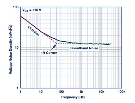
Figure 2. Image courtesy of Analog Devices

 

Above about 100 Hz, the noise power is almost evenly distributed among different frequencies. This region of the noise profile corresponds to the thermal noise of the device. However, as we move to frequencies below 100 Hz, the noise average power increases due to the flicker noise.

Approximating the two distinct regions of the noise profile with straight lines, we can find an intersection point, called the 1/f noise corner frequency (as shown in Figure 2). The corner frequency allows us to determine the dominant noise type of the device (either flicker or thermal) for a given frequency.

Below the 1/f corner frequency, the small signal produced by the sensor can be completely buried in noise. If we could somehow increase the frequency of the sensor output signal to above the corner frequency, we could make a more accurate measurement. This is the basic idea behind the synchronous demodulation technique.

Figure 3 shows how making the measurement at a higher frequency can bring the desired signal out of the device flicker noise.

 

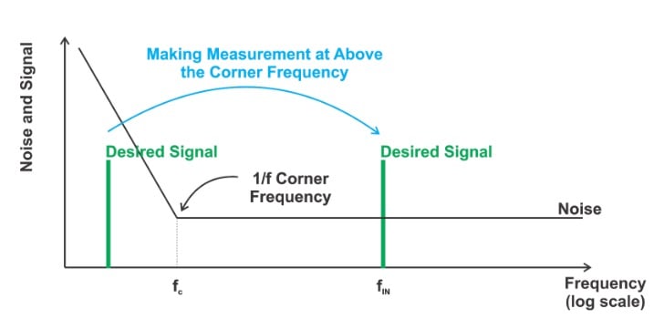
Figure 3

 

The flicker noise may not be a serious problem for the “direct DC” measurement illustrated in Figure 1 because the voice signal displays negligible power at very low frequencies (below about 20 Hz). Additionally, we might be able to customize the internal buffer transistor to decrease its 1/f corner frequency.

However, there are applications where the output signal of the sensor is at much lower frequencies (almost DC) and we need a much more accurate measurement. In this case, the flicker noise of the electronic components can completely bury the signal produced by the sensor and we need techniques such as the synchronous demodulation to circumvent the flicker noise problem.

 

AC Excitation of the Sensor

Figure 4 illustrates the use of an AC signal for measuring a capacitive sensor. In this figure, the variable capacitance C_sense models our capacitive sensor. The input voltage source applies a sine wave with frequency in the 1 kHz-1 MHz range. Depending on the ratio of C_sense to C₂, a voltage signal appears at the input of the op-amp. In this case, the input signal of the op-amp can be chosen to be sufficiently greater than the 1/f corner frequency of the circuit. This is in contrast to the “direct DC” method where the measured signal can be at very low frequencies.

Since the desired signal is far away from the 1/f corner frequency (as shown in Figure 5), the flicker noise is not a limiting factor and we can detect a much smaller signal. 

 

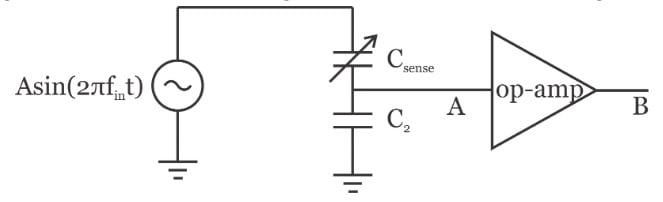
Figure 4 

 

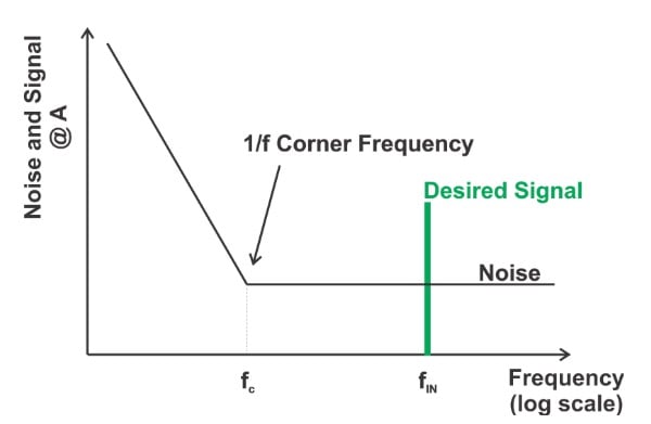
Figure 5

 

At the op-amp output, we have an amplified signal that can be used to determine the value of the variable capacitance; however, we need a band-pass filter (BPF) to reject the noise components and keep only the desired signal. This is depicted in Figure 6.

 

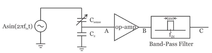
Figure 6

 

Note that the center frequency of the BPF is the same as the input frequency. Assuming that the band-pass filter is ideal, we’ll obtain the desired signal along with the thermal noise that falls in the pass-band of the band-pass filter (Figure 7 below).

 

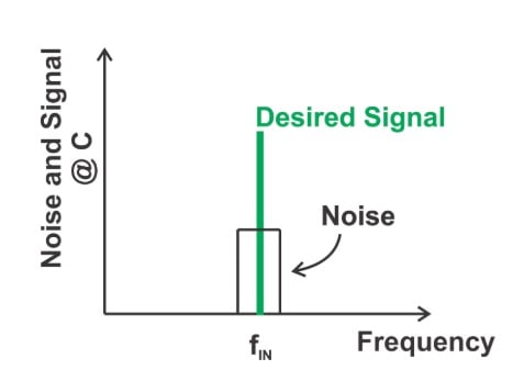
Figure 7

 

Limitations of Using a BPF 

In Figure 6, we need a high-Q band-pass filter to sufficiently suppress the noise and keep the desired signal. A very high-Q filter would allow us to reject most of the noise. However, there are two main problems: First, implementing a high-Q continuous-time band-pass filter can be challenging especially at high frequencies. In fact, as the center frequency of the filter increases, it becomes more and more difficult to achieve a given Q-factor. This is due to the fact that at high frequencies (at about a few hundred MHz), op-amps have limited amplification capability and exhibit non-ideal phase response. You might say that the center frequency of the filter in Figure 6 is in the 1 kHz-1 MHz range and this is not really a high-frequency filter. Well, you’re right, we can have a high-Q filter in this frequency range. However, as we move to higher and higher frequencies, we have to burn more power. In other words, for a given Q-factor, we expect a lower frequency filter to exhibit a lower power consumption. Therefore, it could be more power efficient if the filtering after the op-amp could be performed at a lower frequency.

The second problem with the concept illustrated in Figure 6 is tuning the center frequency of the band-pass filter. Note that the center frequency of an analog continuous-time filter depends on the value of resistors, capacitors, and transconductors. The absolute value of these parameters can vary significantly. As a result, the center frequency of the filter might not be exactly at f_IN. Since the filter has a narrow pass-band, the desired signal might easily fall outside the filter pass-band due to the variations in the filter center frequency. This second problem with the use of a high-Q BPF can be even more challenging than the power efficiency problem discussed in the previous paragraph. Interestingly, if an application requires a high-Q continuous-time band-pass filter, we have to employ a mechanism for tuning the filter center frequency. For example, some integrated band-pass filter applications employ a feedback loop that is conceptually similar to a phase-locked loop to tune the filter center frequency. However, such a system seems too complex and power-hungry for reading a sensor. In the next section, we’ll see that a clever adjustment can achieve the required filtering operation using a low-pass filter rather than a BPF. In this way, we can have a low-power solution that doesn’t need any frequency tuning circuitry. 

 

Synchronous Demodulation

The concept of synchronous demodulation is illustrated in Figure 8. In this figure, a multiplier is placed after the op-amp. 

 

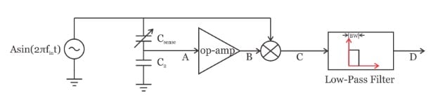
Figure 8

 

Assume that the output signal of the op-amp output is \(v_B(t)=Bsin(2\pi f_{in}t+\phi)\). This signal is multiplied by the input signal \(Asin(2\pi f_{in}t)\) which gives:

 

\[v_C(t)=Asin(2\pi f_{in}t) \times Bsin(2\pi f_{in}t+ \phi)= \frac {1}{2}ABcos(\phi)-\frac {1}{2}ABcos(4\pi f_{in}t+\phi)\]

 

The first term is DC, however, the second term is at twice the input frequency. Hence, a narrow low-pass filter can remove the second term and we have:

 

\[v_D(t)= \frac {1}{2}ABcos(\phi)\]

 

If we assume that the op-amp is not introducing any delay, i.e. \( \phi = 0 \), we obtain \(v_D(t)=\frac {1}{2}AB \). As you can see the output of the low-pass filter is proportional to the amplitude of the signal at node A and can be used to measure the value of \(C_{sense} \). The above method has three advantages:

• The frequency of the sensor output can be chosen to be sufficiently higher than the 1/f corner frequency. 
• The filter operates at the lowest possible frequency and should burn the smallest possible power.
• The filter doesn’t need frequency tuning circuitry.

In the next article of this series, we’ll continue this discussion and take a closer look at the implementation of the synchronous demodulation technique.

 

Conclusion

The “Direct DC” method measures the low-frequency signal produced by a capacitive sensor directly. The accuracy of such low-frequency measurement can be limited because of the flicker noise. To circumvent this problem, we can use an AC signal to excite the sensor. Since the measurement occurs at a frequency above the 1/f corner frequency, the flicker noise is no longer a limiting factor. In this case, we can use a band-pass filter to select the desired signal; however, the use of high-Q bandpass filters can be challenging. Instead, we can synchronously demodulate the measured signal and use a low-pass filter to perform the required filtering. 

To see a complete list of my articles, please visit this page.