Computing Fast Fourier Transforms on the LPC55S69 MCU

NXP’s LPC55S69 microcontroller contains many features that make it suitable for a variety of applications. The LPC55S69 MCU and its PowerQuad unit include unique components — the Biquad and the Transform Engines — that are used to complete various tasks, leaving the main CPU cores free for other things.  

A previous article, Understanding Digital Filtering with Embedded Microcontrollers, explored various widely used methods for filtering and processing data samples in the time domain. For that, it utilized the Biquad engine of the LPC55S69’s PowerQuad unit. 

This article investigates the Transform Engine, another part of the PowerQuad, which enables the LPC55S69 MCU to compute a Fast Fourier Transform (FFT).

 

Understanding Discrete Fourier Transforms

When dealing with everyday measurements such as lengths and temperatures, a set of tools exists to determine the size and temperature of the particular thing being measured. For time-domain signals, the choice of measuring tool might not be so apparent. Consider the following signal example given in Figure 1.

 

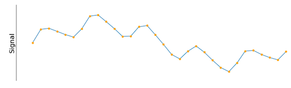
Figure 1. An input signal sampled at a constant interval.

 

How can this signal be measured, understood, and described? Possible choices could be the amplitude, the frequency, or several values calculated with methods from statistics. One way to begin is by gauging the signal of interest against a known cosine wave, shown in Figure 2.

 

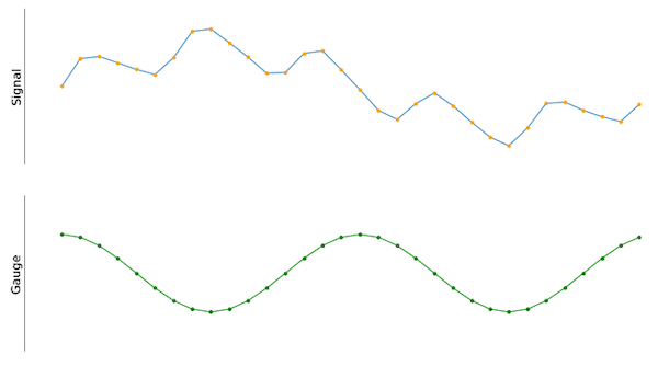
Figure 2. The input signal next to a cosine gauge signal. Both have the same number of samples.

 

Because the amplitude and frequency of the cosine wave can be easily fixed and therefore identified, it's possible to compare the cosine wave to the input signal. If done correctly, the resulting value of the dot-product between the input signal and the cosine wave quantifies how much the input signal correlates to the gauge. For that, it's reasonable to think of the input and gauge signal as discrete input arrays of the same length, and it becomes easy to calculate the dot-product. 

The result is a scalar, and its magnitude is proportional to how well the input signal correlates to the cosine gauge signal. The dot-product operation boils down to many multiply and add operations — the same operation discussed in Understanding Digital Filtering with Embedded Microcontrollers.

This method quickly yields good results. There is, however, a particular case that does not work when applying this method. If the input signal is a cosine wave with the same frequency as the gauge, but with its phase shifted by 90 degrees with respect to the gauge, the output of the aforementioned method will be zero.  By visual inspection, it appears that there is still a correlation between the gauge and the input signal but there is detail that we need to account for.

 

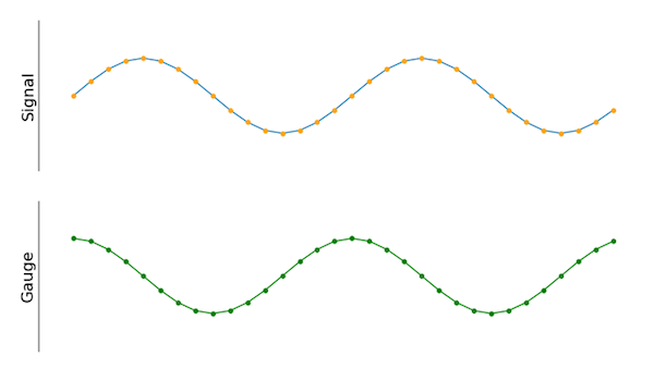
Figure 3. The new gauge signal is phase-shifted by 90 degrees compared to the old one.

 

This behavior could be compared to measuring the “length” of a thin strip of paper. When using a ruler to determine the length of one side of the paper strip, the paper might be 10 inches long and one inch wide. Both numbers are correct, but the ruler had to be rotated by 90 degrees to obtain both measurements.  Both numbers are technically correct and we can use them together to get a true “size” (length and width) of our piece of paper. To overcome this problem in terms of our input signal, a second gauge can be used, as seen in Figure 4. 

 

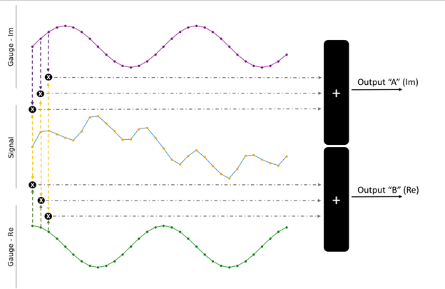
Figure 4. Both gauge signals can be used to better quantify the input signal.

 

The only difference between the two gauges (shown in purple and green) is the 90-degree phase shift. In the previous analogy, this is the equivalent of rotating the ruler. The dot-product is calculated between the input signal and each of the gauges to obtain the final output. This yields results in two values A and B, each containing how well the input correlates to one of the gauges. Typically, they are considered as a single complex number:

output = B + i * A

The next step is to compare the input signal to a range of gauges with different frequencies (Figure 5).

 

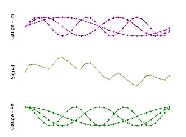
Figure 5. Multiple gauges can be applied as well. The green ones are shifted by 90 degrees compared to the purple ones.

 

As the image shows, the final result incorporates a few different gauges. The imaginary portion (shown in purple) is phase shifted by 90 degrees compared to the green signals (real part), just like in the two-gauge example shown above. There is no limit to the number of different gauges. 

Using this technique — called the Discrete Fourier Transform (DFT) — yields the generation of a spectrum of outputs at all the frequencies of interest for a problem. It's possible to state the technique mathematically as follows:

 

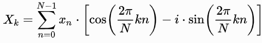
Equation 1. The mathematical description of the DFT.

 

Where N is the number of samples in the input signal and k is the frequency of the (co)sine reference gauges.

 

Fast Fourier Transform (FFT) Limitations

The FFT is a numerically efficient way of computing the DFT that requires fewer multiply and add operations compared to the method discussed above. However, there are a few restrictions to the input:

1. The length of the input must be a power of two.
2. Arbitrary input lengths and frequency spacing in the output are not allowed. The output bins are spaced by the input signal’s sample rate divided by the number of samples in the input. If the input is, for example, a 256-point signal sampled at 48 kHz, the output arrays correspond to frequencies spaced at 187 Hz (48.000 divided by 256).
3. When the input consists of real numbers (for example, samples obtained from an ADC), the output is symmetric. If the input, for example, consists of 64 samples, the FFT result will also consist of 64 complex numbers. However, the second half of the output array contains the complex conjugates of the first half.

 

Using the PowerQuad FFT Engine

The math behind DFT/FFT operations can be performed by simple multiply and add operations, which is ideal for outsourcing the mathematical operations to a dedicated coprocessor, such as the PowerQuad on the LPC55S69 MCU. Because of this, the main CPU cores are free to work on other tasks. 

Utilizing the PowerQuad FFT engine is a simple process, and the official SDK comes with example projects that demonstrate the coprocessing features. One example in particular, called powerquad_transform, demonstrates the FFT calculation process.

The powerquad_transform.c file contains several functions that test the different FFT engine modes. One of them is the PQ_RFFTFixed16Example function. This example initializes the PowerQuad to accept 16-bit integer data. Floating-point data must be converted to fixed-point values beforehand, as the PowerQuad transform engine only supports integers.

FILTER_INPUT_LEN defines the number of input samples. The output array is twice the length because it needs to store the real and imaginary parts of the resulting values.

 

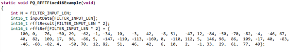
Figure 6. This part of the code defines the test-data and the expected results.

 

The last array contains test data for verifying the result. Note how the second half of the array contains the complex conjugates as stated above. Furthermore, the conjugates are not equal (e.g. the pair 76,-50, and 77,49). Anyway, once the data got initialized, the following data structure is used to configure the PowerQuad:

 

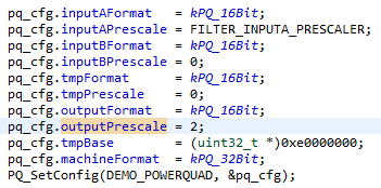
Figure 7. This part of the example program configures and initializes the PowerQuad unit.

 

It's necessary to downscale the input to prevent the algorithm from overflowing. This process happens in the second line in the image above. FILTER_INPUTA_PRESCALER is set to five because there are 32 (two to the power of five) samples. The pre-scaling is another hardware feature of the PowerQuad, and it is likely the reason for the imprecision observed in the expected test results.

Once everything is set up, the location of the input and output areas is passed to the PowerQuad unit, which happens in the PQ_transformRFFT function. This method sets a few configuration registers and starts the PowerQuad by writing to the control register. In this example, the CPU waits for the PowerQuad to finish. Waiting is not always necessary, and the PowerQuad can perform calculations asynchronously while the CPU performs other tasks.

 

Utilize the PowerQuad for Mathematical Operations

The PowerQuad is a coprocessor for complex mathematical operations available on various devices of the LPC5500 MCU series. It includes a special engine for efficiently calculating FFTs, which can be done independently from the main CPU cores. The SDK for the LPC55S69 MCU contains examples of how to set up and use the PowerQuad.

NXP’s Community Page contains extensive information, discussions, and articles centered around the LPC55S69 MCU.

Industry Articles are a form of content that allows industry partners to share useful news, messages, and technology with All About Circuits readers in a way editorial content is not well suited to. All Industry Articles are subject to strict editorial guidelines with the intention of offering readers useful news, technical expertise, or stories. The viewpoints and opinions expressed in Industry Articles are those of the partner and not necessarily those of All About Circuits or its writers.