What is Hysteresis? An Introduction for Electrical Engineers

As a technical term, hysteresis first referred to a phenomenon exhibited by magnetic materials. It has since been incorporated into many fields of study—if you search for “hysteresis” in a collection of reference works, you’ll find entries in dictionaries and encyclopedias not only for engineering but also for physics, geography, environmental sciences, economics, and even dentistry.

A concept whose use has expanded and diversified in this way isn’t likely to have a concise, comprehensive definition available, so defining hysteresis will be the first task of this article. We’ll focus on hysteresis as a property of materials, components, and circuits that figure prominently in the work performed by electrical engineers.

 

Hysteresis Defined

Despite the differences between them, the following excerpts from reference entries all convey key characteristics of hysteresis. All of them will help you build a robust mental model for this important phenomenon.

• “A delay in the change of an observed effect in response to a change in the mechanism producing the effect” —Oxford Dictionary of Electronics and Electrical Engineering.
• “A lagging effect from an expected value due to a resistance such as friction” —Oxford Dictionary of Chemical Engineering.
• “A situation in which the equilibrium of a system depends upon the history of the system” —Oxford Dictionary of the Social Sciences.
• “A phenomenon in which two physical quantities are related in a manner that depends on whether one is increasing or decreasing in relation to the other” —Oxford Dictionary of Physics.

Interestingly, the entry from the social sciences dictionary seems to me like the best starting point.

When describing the relationship between two quantities, we can usually say that a particular input value corresponds to a particular output value. For example, an amplifier has an input voltage and an output voltage, and these are related by the gain (which in real life would be a function of frequency rather than a constant). If we ignore non-idealities such as saturation, V_OUT always equals gain times V_IN.

However, if the relationship is hysteretic, we can’t say that a particular input value always produces a particular output value. Instead, the input-to-output relationship depends on the history of the system, as the classic hysteresis curve in Figure 1 illustrates.

 

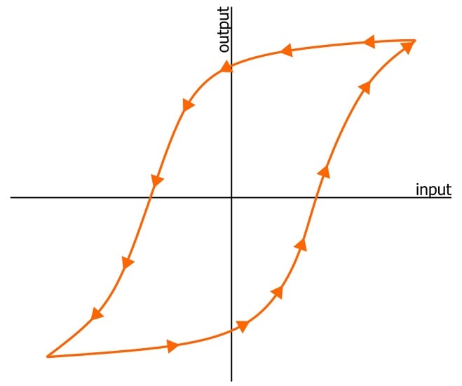
Figure 1. A simple hysteresis curve.

 

The horizontal axis is the input, and the vertical axis is the output. If you choose an input value that lies within the enclosed portion of the hysteresis curve, what’s the corresponding output value? There’s no clear answer to this question, as Figure 2 demonstrates.

 

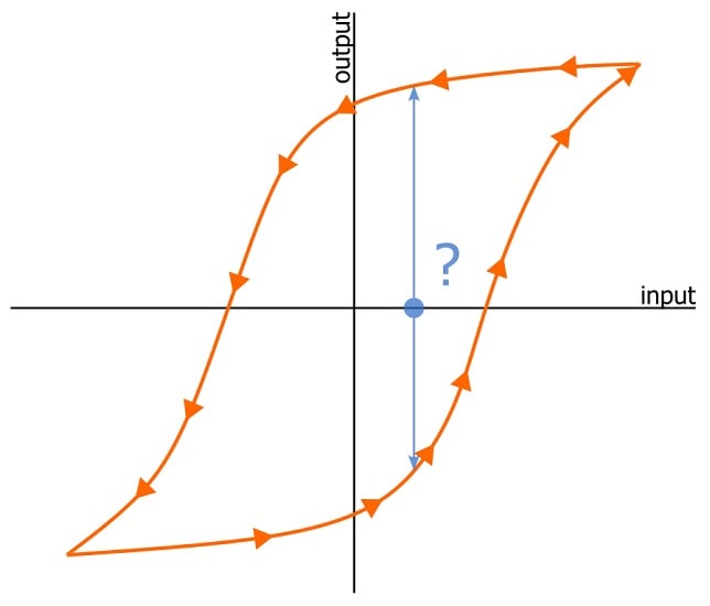
Figure 2. Input value enclosed by a hysteresis curve. The output value is indeterminate.

 

Hysteresis and Relative Movement

In order to properly answer questions about which output value corresponds to a given input value, we need additional information about the history of the system. Here, the definition from the Dictionary of Physics is especially helpful: in the presence of hysteresis, the input-to-output relationship depends on whether the input is increasing or decreasing relative to the output. Increasing and decreasing imply movement, movement—as Aristotle pointed out—presupposes time, and change over time is recorded as history.

Saying that a hysteretic system’s current state depends on the system’s history is therefore a generalized, less technical way of saying that hysteresis makes an input-to-output relationship dependent on relative movement. If the input is currently increasing relative to the output (Figure 3), we find the output value using the curve marked by upward arrows; if the input is currently decreasing relative to the output (Figure 4), we find the output value using the curve marked by downward arrows.

 

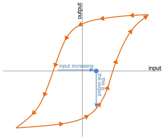
Figure 3. Hysteresis curve with input increasing relative to the output.

 

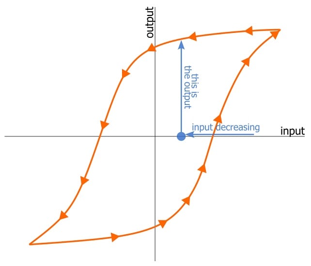
Figure 4. Hysteresis curve with input decreasing relative to the output.

 

The “Digital” Hysteresis Curve

If we stretch and fold the smooth hysteresis curves shown above into idealized rectangular transfer functions, we get Figure 5. Being accustomed to the on/off type of hysteresis action found in comparator circuits, I personally find this “digital” version of the hysteresis curve more intuitive than the gradual transitions we examined earlier.

 

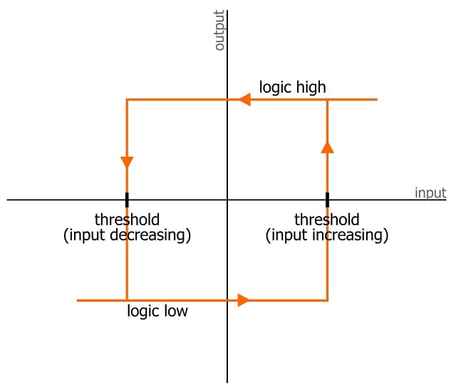
Figure 5. Hysteresis as a rectangular transfer function instead of a curve.

 

If this circuit had no hysteresis, the transfer function would look like a step function, and there would be only one threshold. If the input were to the left of that single threshold, the output would be logic-low; if it were to the right of the threshold, the output would be logic-high.

When we add hysteresis, we create an indeterminate region bounded by two different thresholds. If the input value is outside the square, there’s no indeterminacy: the output will be logic low if the input is to the left of the square and logic high if the input is to the right of the square. If the input value is somewhere inside the square, the output depends on the system’s history.

The following sequence of events conveys the history-dependent (or, if you prefer, relative-movement-dependent) relationship created by hysteresis:

1. The input value is below the lower threshold. The output is logic-low.
2. The input crosses the lower threshold and moves into the square. Since the input is increasing, the output doesn’t change.
3. The output remains logic-low until the input reaches the higher threshold. The output then transitions to logic-high.
4. The input increases above the higher threshold. The output remains logic-high.
5. The input starts to decrease and eventually reaches the higher threshold. The output remains logic-high.
6. The input is now inside the square, but the output is still logic-high. Previously, the input was inside the square, and the output was logic-low. The output state is different because of the system’s history: previously the input was inside the square and increasing, but now it’s inside the square and decreasing.
7. The input reaches the lower threshold. Now the output transitions to logic-low.

 

Up Next

In this article, we introduced the foundational principles of hysteresis and examined visual representations of a hysteretic system’s history-dependent nature. Next time, we’ll explore the theoretical differences between rate-dependent and rate-independent hysteresis.

 

Background of the featured image used courtesy of Adobe Stock; all other images used courtesy of Robert Keim