 Facebook
 Google
 GitHub
 Linkedin
Solving Simultaneous Equations: The Substitution Method and the Addition Method
What are Simultaneous Equations and Systems of Equations?
The terms simultaneous equations and systems of equations refer to conditions where two or more unknown variables are related to each other through an equal number of equations.
Example:
For this set of equations, there is but a single combination of values for x and y that will satisfy both.
Either equation, considered separately, has an infinitude of valid (x,y) solutions, but together there is only one. Plotted on a graph, this condition becomes obvious:
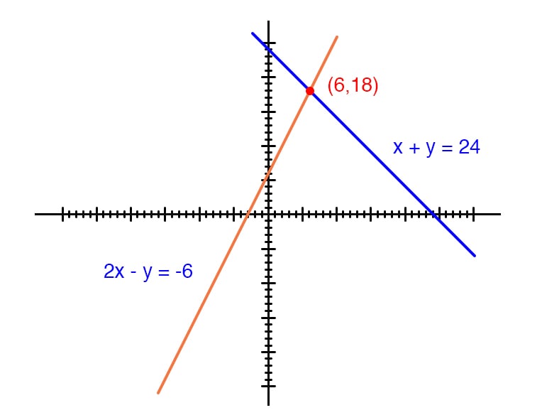
Each line is actually a continuum of points representing possible x and y solution pairs for each equation.
Each equation, separately, has an infinite number of ordered pair (x,y) solutions. There is only one point where the two linear functions x + y = 24 and 2x - y = -6 intersect (where one of their many independent solutions happen to work for both equations), and that is where x is equal to a value of 6 and y is equal to a value of 18.
Usually, though, graphing is not a very efficient way to determine the simultaneous solution set for two or more equations. It is especially impractical for systems of three or more variables.
In a three-variable system, for example, the solution would be found by the point intersection of three planes in a three-dimensional coordinate space—not an easy scenario to visualize.
Solving Simultaneous Equations Using The Substitution Method
Several algebraic techniques exist to solve simultaneous equations.
Perhaps the easiest to comprehend is the substitution method.
Take, for instance, our two-variable example problem:
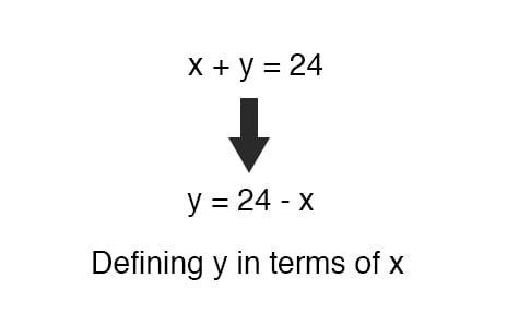
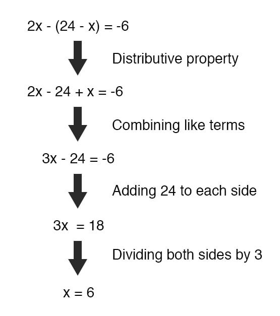
In the substitution method, we manipulate one of the equations such that one variable is defined in terms of the other:
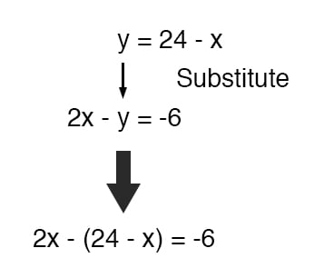
Then, we take this new definition of one variable and substitute it for the same variable in the other equation.
In this case, we take the definition of y, which is 24 - x and substitute this for the y term found in the other equation:
Now that we have an equation with just a single variable (x), we can solve it using “normal” algebraic techniques:
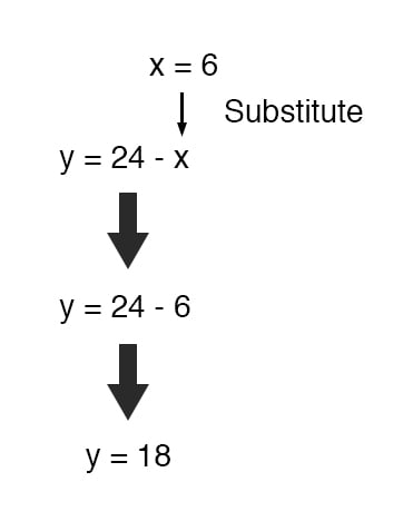
Now that x is known, we can plug this value into any of the original equations and obtain a value for y.
Or, to save us some work, we can plug this value (6) into the equation we just generated to define y in terms of x, being that it is already in a form to solve for y:
Applying the substitution method to systems of three or more variables involves a similar pattern, only with more work involved.
This is generally true for any method of solution: the number of steps required for obtaining solutions increases rapidly with each additional variable in the system.
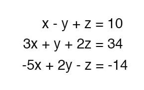
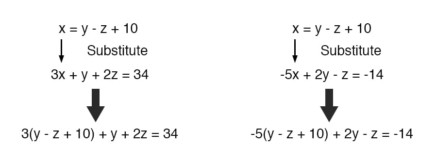
To solve for three unknown variables, we need at least three equations. Consider this example:
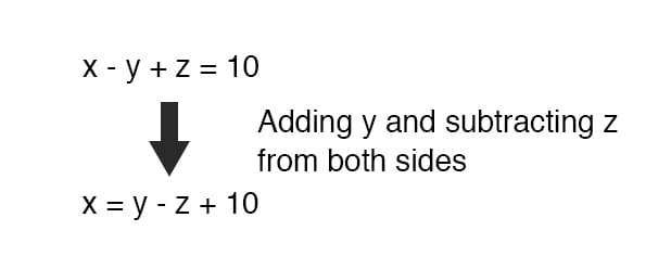
Being that the first equation has the simplest coefficients (1, -1, and 1, for x, y, and z, respectively), it seems logical to use it to develop a definition of one variable in terms of the other two.
Solve for x in terms of y and z:
Now, we can substitute this definition of x where x appears in the other two equations:
Reducing these two equations to their simplest forms:
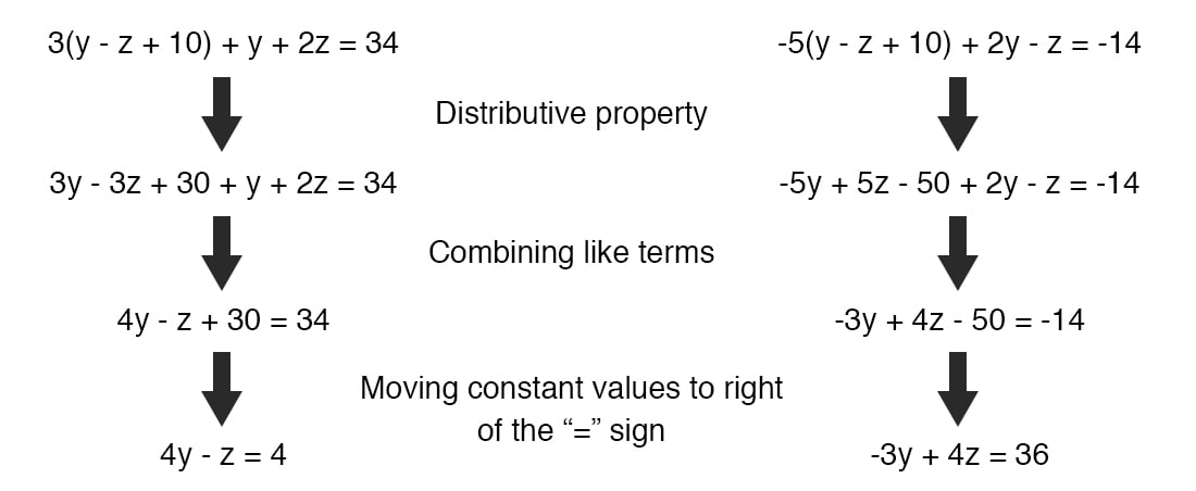
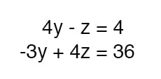
So far, our efforts have reduced the system from three variables in three equations to two variables in two equations.
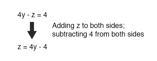
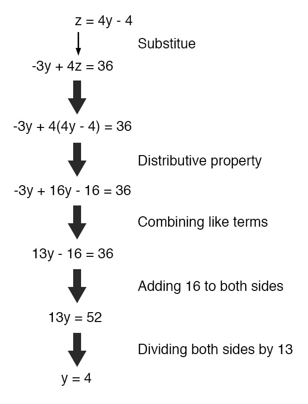
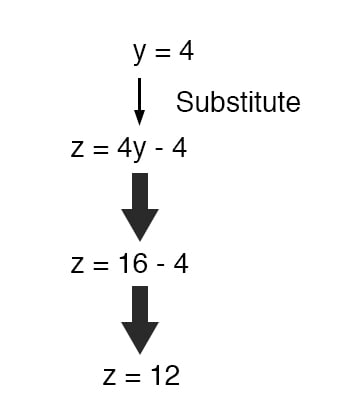
Now, we can apply the substitution technique again to the two equations 4y - z = 4 and -3y + 4z = 36 to solve for either y or z. First, I’ll manipulate the first equation to define z in terms of y:
Next, we’ll substitute this definition of z in terms of y where we see z in the other equation:
Now that y is a known value, we can plug it into the equation defining z in terms of y and obtain a figure for z:
Now, with values for y and z known, we can plug these into the equation where we defined x in terms of y and z, to obtain a value for x:
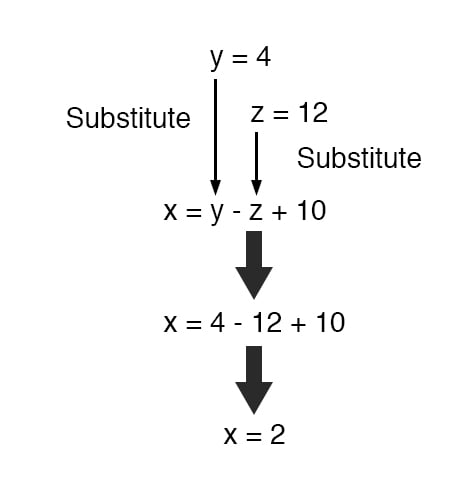
In closing, we’ve found values for x, y, and z of 2, 4, and 12, respectively, that satisfy all three equations.
Solving Simultaneous Equations Using The Addition Method
While the substitution method may be the easiest to grasp on a conceptual level, there are other methods of solution available to us.
One such method is the so-called addition method, whereby equations are added to one another for the purpose of canceling variable terms.
Let’s take our two-variable system used to demonstrate the substitution method:
One of the most-used rules of algebra is that you may perform any arithmetic operation you wish to an equation so long as you do it equally to both sides.
With reference to addition, this means we may add any quantity we wish to both sides of an equation—so long as its the same quantity—without altering the truth of the equation.
An option we have, then, is to add the corresponding sides of the equations together to form a new equation.
Since each equation is an expression of equality (the same quantity on either side of the = sign), adding the left-hand side of one equation to the left-hand side of the other equation is valid so long as we add the two equations’ right-hand sides together as well.
In our example equation set, for instance, we may add x + y to 2x - y, and add 24 and -6 together as well to form a new equation.
What benefit does this hold for us? Examine what happens when we do this to our example equation set:
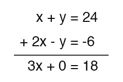
Because the top equation happened to contain a positive y term while the bottom equation happened to contain a negative y term, these two terms canceled each other in the process of addition, leaving no y term in the sum.
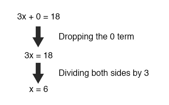
What we have left is a new equation, but one with only a single unknown variable, x! This allows us to easily solve for the value of x:
Once we have a known value for x, of course, determining y‘s value is a simply matter of substitution (replacing x with the number 6) into one of the original equations.
In this example, the technique of adding the equations together worked well to produce an equation with a single unknown variable.
What about an example where things aren’t so simple? Consider the following equation set:
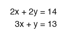
We could add these two equations together—this being a completely valid algebraic operation—but it would not profit us in the goal of obtaining values for x and y:
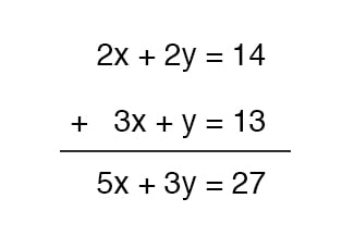
The resulting equation still contains two unknown variables, just like the original equations do, and so we’re no further along in obtaining a solution.
However, what if we could manipulate one of the equations so as to have a negative term that would cancel the respective term in the other equation when added?
Then, the system would reduce to a single equation with a single unknown variable just as with the last (fortuitous) example.
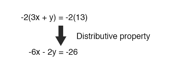
If we could only turn the y term in the lower equation into a - 2y term, so that when the two equations were added together, both y terms in the equations would cancel, leaving us with only an x term, this would bring us closer to a solution.
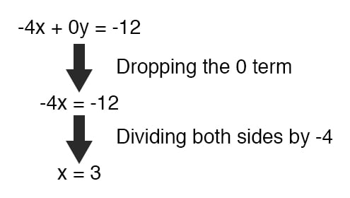
Fortunately, this is not difficult to do. If we multiply each and every term of the lower equation by a -2, it will produce the result we seek:
Now, we may add this new equation to the original, upper equation:
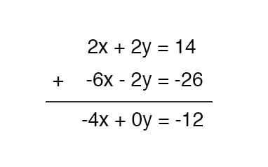
Solving for x, we obtain a value of 3:
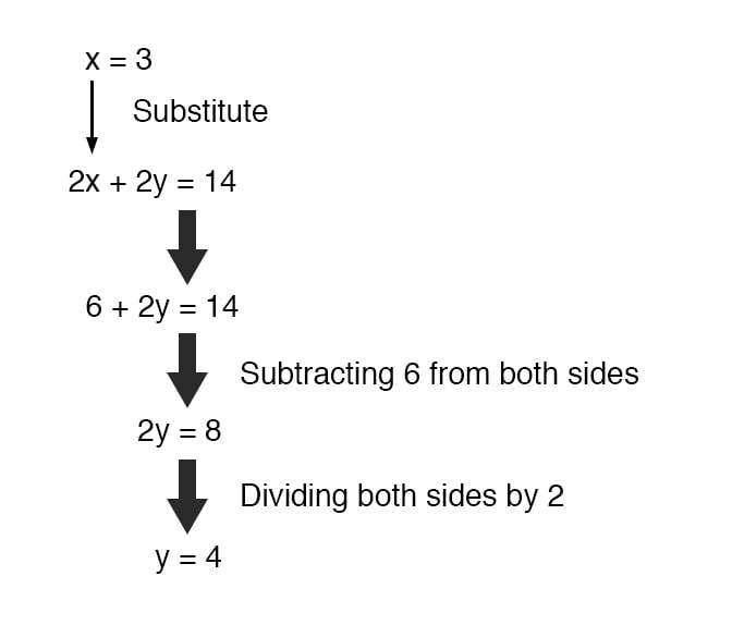
Substituting this new-found value for x into one of the original equations, the value of y is easily determined:
Using this solution technique on a three-variable system is a bit more complex.
As with substitution, you must use this technique to reduce the three-equation system of three variables down to two equations with two variables, then apply it again to obtain a single equation with one unknown variable.
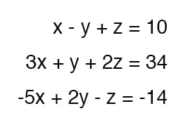
To demonstrate, I’ll use the three-variable equation system from the substitution section:
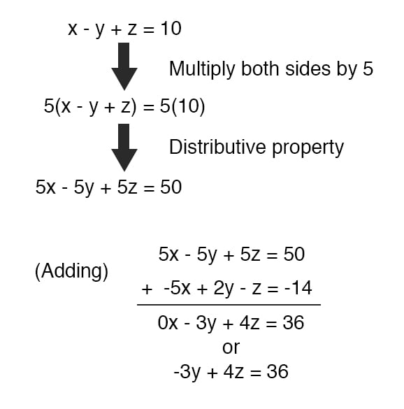
Being that the top equation has coefficient values of 1 for each variable, it will be an easy equation to manipulate and use as a cancellation tool.
For instance, if we wish to cancel the 3x term from the middle equation, all we need to do is take the top equation, multiply each of its terms by -3, then add it to the middle equation like this:

We can rid the bottom equation of its -5x term in the same manner: take the original top equation, multiply each of its terms by 5, then add that modified equation to the bottom equation, leaving a new equation with only y and z terms:
At this point, we have two equations with the same two unknown variables, y and z:
By inspection, it should be evident that the -z term of the upper equation could be leveraged to cancel the 4z term in the lower equation if only we multiply each term of the upper equation by 4 and add the two equations together:
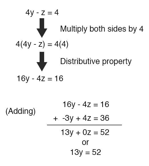
Taking the new equation 13y = 52 and solving for y (by dividing both sides by 13), we get a value of 4 for y.
Substituting this value of 4 for y in either of the two-variable equations allows us to solve for z.
Substituting both values of y and z into any one of the original, three-variable equations allows us to solve for x.
The final result (I’ll spare you the algebraic steps since you should be familiar with them by now!) is that x = 2, y = 4, and z = 12.
RELATED WORKSHEETS:


Simplify and solve the following set of simultaneous equations a) 4( 𝑥 + 3𝑦) – 2( 4𝑥 + 3𝑧) – 3( 𝑥 − 2𝑦 − 4𝑧 = 17 )
2(4𝑥 − 3𝑦) + 5( 𝑥 − 4𝑧) + 4( 𝑥 − 3𝑦 + 2𝑧) = 23
3 (𝑦 + 4𝑧) + 4 (2𝑥 − 𝑦 − 𝑧 )+ 2 (𝑥 + 3𝑦 − 2𝑧) = 5