 Facebook
 Google
 GitHub
 Linkedin
An Introduction to Control Systems: Designing a PID Controller Using MATLAB’s SISO Tool
Control systems engineering requires knowledge of at least two basic components of a system: the plant, which describes the mathematically described behavior of your system, and the output, which is the goal you are trying to reach.
Introduction
Control systems engineering requires knowledge of at least two basic components of a system: the plant, which describes the mathematically modeled behavior of your system, and the output which is the goal you are trying to reach. A control system which has become commonplace in the automotive industry is the cruise control system: an output is programmed by the driver, and the control system has to manage all of the vehicle readings in order to maintain velocity.
Because the road we drive on has imperfections, sometimes the system will have to accelerate or decelerate automatically. If you’ve ever used this feature on a car, you may have noticed that the car tends to keep a very smooth pace on the velocity you’ve chosen - it doesn’t abruptly accelerate or decelerate. This means that the vehicle’s control system is first given a desired output, then manages errors of the actual output by compensating for the input (for example, by how much fuel is provided to the engine).
Before solving for a system, we will briefly analyze the components and behavior of a system (uncompensated) and then the individual components of a PID (proportional-integral-derivative) controller. The final step would be to bring these two together and design a PID controller that will compensate the originally observed system. It is important to know that PID controllers are not the only type of compensation a designer can apply to system, but it's a great place to start and learn some of the universal characteristics that will stay true in other methods.
Note: In this tutorial we will be analyzing analog systems under ideal conditions (no noise or disturbance) and all or most the mathematical analysis will done via MATLAB.
Observing a System
A system can be made up of various components arranged in equally various ways; but we will begin by analyzing the components and functionality of a classical closed-loop sytem (Figure 1).
.png)
Figure 1 - An example block diagram of a single-input single-output system closed loop system.
- Input: r - An input is some sort of reference value that should have a direct correlation with the system’s output. This doesn’t necessary translate directly to a voltage/power source, but rather a setting or switch that will connect a voltage/power source to the system. In the system example that we will analyze later, our input signal will be a unitary step.
- Controller: C - In our case, this is the PID controller that we will design. It is positioned before the plant that we are compensated for and just after the junction of the input signal and feedback.
- Plant: G - This is all of your subsystems mathematically expressed as a transfer function. If what you are attempting to control is a DC motor, then the plant is in fact, your DC motor. You input will cause the plant to react in a way that will supply an output value that is ideally close to your input.
- Output: y - This reading is the actual system’s response to our desired response (the input) which has passed through our assembled system (plant). The performance of the system is judged by the comparison of the output to the input, given that certain errors will occur and have been taken into account as acceptable.
- Feedback: H - In a system’s equivalent block diagram (see Figure 1), the feedback line introduces the output of the system into the input. What this means is that any discrepancies between the output (actual response) and input (desired response) can be measured - in other words, the error between the input and output is what is introduced to the controller. Our system's error is then equal to: input - output x H; if the system has a unitary feedback (meaning that H = 1), then our error is simply input minus the output. This will be an important idea to remember when we move onto describing how each facet of the PID controller works.
- It is important to note that the transfer function for the complete loop in Figure 1 could be further simplified into just one block with a single input and single output by the use of the closed loop transfer function:
\[Closed-Loop(s)=\frac{C(s)\cdot G(s)}{1+C(s)\cdot G(s)\cdot H(s)}\]
PID Control Definition
A PID controller is actually a three part system:
- Proportional compensation: the main function of the proportional compensator is to introduce a gain that is proportional to the error reading which is produced by comparing the system's output and input.
- Derivative compensation: in a unitary feedback system, the derivative compensator will introduce the derivative of the error signal multiplied by a gain \[K_{D}\]. In other words, the slope of the error signal's waveform is what will introduced to the output. Its main purpose is that of improving the transient response of the overall closed-loop system.
- Integral compensation: in a unitary feedback system, the integral compensator will introduce the integral of the error signal multiplied by a gain \[K_{I}\]. This means that the area under the error signal's curve will be affecting the output signal. We will prove this later, but it is important to note that this facet of the controller will improve the steady-state error of overall closed-loop system.
| Compensation | Time Domain | S-Domain |
|---|---|---|
| Proportional | \[K_{P} e(t)\] | \[K_{p}\] |
| Derivative | \[K_{D}\frac{d}{dt}e(t)\] | \[K_{D}s\] |
| Integral | \[K_{I}\int_{0}^{t}e(x)d(x)\] | \[\frac{K_{I}}{s}\] |
Therefore, a PID controller can be mathematically described as:
| Compensation | Time Domain | S-Domain |
|---|---|---|
| PID Controller | \[K_{P} e(t)+K_{D}\frac{d}{dt}e(t)+K_{I}\int_{0}^{t}e(x)d(x)\] | \[K_{P} +K_{D}s+\frac{K_{I}}{s}=\frac{K_{P}s+K_{D}s^2+K_{I}}{s}\] |
For no reason other than simplicity, one can see why the s-domain is exclusively used when analyzing or designing analogous systems - working with fractions is always easier than doing integration and/or derivatives. If we now take what we have described as a PID controller and apply it to Figure 1, our block diagram will now resemble something like what you see in Figure 1.1 below.
.png)
Figure 1.1 - Our "C" block is essentially everything contained within the red box: the summation of proportional, derivative and integral compensations to the system.
Output Characteristics
Now that we know what a system is made of and how we will applying our PID controller, we can start to talk about the characteristics of our output signal (afterall, this is what we're monitoring and attempting to change)
Important Equations
Output analysis:
| Characteristic | Equation | Description |
| General Equation (2nd-order) | \[G(s)=\frac{\omega_{n}^{2}}{s^{2}+2\zeta \omega_{n}s+\omega_{n}^{2}}\] | This general equation will help describe the behavior of a typical second-order function with no zeros. However, not all transfer functions are or will be second-order and many will contain zeros. In these cases it is required to do a partial fractions analysis to determine the error between using the second-order equations on a higher-order system. (Note: we will assume the error is acceptable for the example used later in this article). |
| Overshoot (percent) | \[pOS=e^{-(\zeta \pi /\sqrt{1-\zeta ^{2}})}\ast 100\] | This value will describe the percent at which the output's waveform overshoots (or surpasses) it's final/steady-state value. It is expressed as a percent of the the final value. |
| Damping Ratio | \[\zeta=\frac{-\ln(pOS/100)}{\sqrt{\pi^{2}+ln^{2}(pOS/100)}}\] | It is important to take note that the equation for the damping ratio is solely dependant on the overshoot. The ratio will describe if a system is is undamped (equal to 0), underdamped (between 0 and 1), critically damped (equal to 1), or overdamped (greater than 1). |
| Peak-Time | \[T_{p}=\frac{\pi}{\omega_{n}\sqrt{1-\zeta^2}}\] | This is the time (in seconds) for the waveform to reach its maximum, or peak, value. |
| Settling-Time | \[T_{s}=\frac{4}{\zeta \omega _{n}}\] | The time it takes for the waveform to settle within +/- 2% of the final/steady-state value. Because oscillations may continue indefinitely (albeit minor), this does not require the waveform to settle absolutely. |
Steady-state error Analysis:
\[e(\infty )=e_{step}(\infty )=\frac{1}{1+K_{p}}\] where \[K_{p}=\lim_{s \to 0}G(s)\]
\[e(\infty )=e_{ramp}(\infty )=\frac{1}{K_{v}}\] where \[K_{v}=\lim_{s \to 0}s\cdot G(s)\]
\[e(\infty )=e_{parabola}(\infty )=\frac{1}{K_{a}}\] where \[K_{a}=\lim_{s \to 0}s^{2}\cdot G(s)\]
Graphical Representations:

Figure 1.2 - The plot provides a visualization of how different damping ratios affect a system's output (in response to a step). This also shows a the direct correlation between a system's damping ratio and percent overshoot (the smaller the damping ratio, the larger the overshoot).
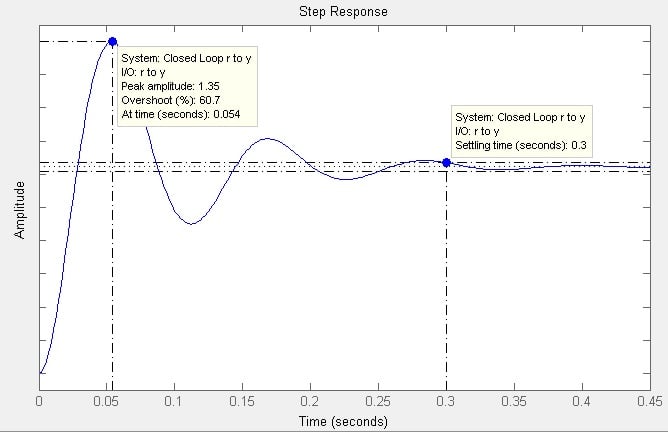
Figure 1.3 - An example of a systems response to a step input. Using MATLAB SISO Tool's analysis allows for the user to display characteristics of the response - in this case: peak-time, overshoot, and settling-time.
Controller Design in Matlab
There are several improvements we need to do once we have our transfer function of the component (or plant) whose response needs to be improved. MATLAB includes many “engineering toolboxes” that enable engineers to create, analyze and simulate a variety of different projects. In our case, MATLAB has included the Control Systems Toolbox which includes several functions tailored for control systems engineering. They’ve also included the SISO (single-input single-output) tool, a GUI that allows for interactive system analysis and control design. Two of the best aspects of the SISO tool approach are:
-
How changes in the transfer function’s poles and zeros alter the root locus and bode plots in live response. The changes in gain can also be instantly reflected in the system’s step response.
-
Specifying the design requirements will create visual limitations on the graphs to help the user set and find appropriate gains. This is done by right-clicking on the SISO tool root locus plot and selecting ‘Design Requirements’. You then chose the type of characteristic you want to set and define its limits. This will provide you with a defined border limit and a shaded ‘invalid’ area (orange shade). It is important that as a designer, you keep a list of your priorities and note the specifications that are of most importance.
Example System Transfer Function:
\[G(s)=\frac{K(s+8)}{(s+3)(s+6)(s+10)}\]
Design Requirements:
- An overshoot of no more than 20%
- Peak-time (Tp) that is no more than two-thirds that of uncompensated system. (refer to equations)
- Zero steady-state error for a step-input (refer to equations)
Sectioned MATLAB Script
%%  Define our Plant

n=poly([-8]);  %defining our numerator
d=poly([-3 -6 -10]);  %defining our denominator
Ps=tf(n,d)  %tf is a function that calls for a predefined numerator and
            %denominator value to create a transfer function
Ts=feedback(Ps,1) %the feedback function will automatically provide you
                  %with the closed loop transfer function while defining
                  %your plant as the first variable, and your feedback as
                  %your second variable

% Once you click on "Run Section" you will note that values have appeared
% in your Workspace and a transfer function as been printed in your
% Command Window.

%%  Run SISO tool to analyze Plant transfer function

sisotool(Ps)  %Note that we are running sisotool on the open-loop TF

%%  Apply gain & analyze system response

% At this point you can either export your gain (K) value or you can
% manually enter and save the value in your workspace.
K=116.5;  %K as given through siso analysis
Ps1=K*Ps  %Muliplying K with plant
Ts1=feedback(Ps1,1)  %This will provide the closed loop transfer function
                     %where the feedback line has a value of just 1
                     %(nothing contained in feedback - unitary feedback)
stepinfo(Ts1)  %stepinfo will print detailed step response data
step(Ts,Ts1);  %will provide a graph of the step response for visual analysis

%% Calculate Goal Peak-Time
Tp=0.2978;  %value of Tp that I found in previous section from stepinfo
Tp_goal=Tp*(2/3)  %printing my goal peak time in command window

pOS = 20;
dr=-log(pOS/100)/sqrt(pi^2+(log(pOS/100))^2); % OS to Damping Ratio eq.
w=pi/(Tp_goal*sqrt(1-(dr^2)))  % Peak Time and DR to find freq.

%%  Apply PD compensation

% Here we run sisotool again, this time on Ps1 instead of Ps.
% We will now add an additional design characteristic - our goal peak-time
% Refer to peak-time equation to find settling-time equivalent

sisotool(Ps1)

%%  Export the PD compensator for analysis

PD=C  %Only run this section once to ensure that PD is not overwritten with
      %another C value from SISO tool
Ps2=Ps1*PD
Ts2=feedback(Ps2,1)
stepinfo(Ts2)
step(Ts,Ts1,Ts2)

%%  Apply PID compensation
% As before, we will run sisotool, this time on Ps2 and finalize our PID

sisotool(Ps2)

%%  Export the PID compensator value for analysis

PID=C  % This will carry the value of our new C and attach it to PID
Ps3=Ps2*PID  % muliply the integrator to the PD
Ts3=feedback(Ps3,1)
stepinfo(Ts3)
step(Ts,Ts1,Ts2,Ts3)

%% Finally we will calculate our steady-state error (refer to equations)

kp=dcgain(Ps3); % dcgain is a function that will carry out our limit s->0
ess=1/(1+kp) % this is the equation for the steady state error for a stepCommand Window Prompts
Ps =

            s + 8
  --------------------------
  s^3 + 19 s^2 + 108 s + 180

Continuous-time transfer function.


Ts =

            s + 8
  --------------------------
  s^3 + 19 s^2 + 109 s + 188

Continuous-time transfer function.


Ps1 =

        116.5 s + 932
  --------------------------
  s^3 + 19 s^2 + 108 s + 180

Continuous-time transfer function.


Ts1 =

          116.5 s + 932
  -----------------------------
  s^3 + 19 s^2 + 224.5 s + 1112

Continuous-time transfer function.


ans =

        RiseTime: 0.1330
    SettlingTime: 0.7119
     SettlingMin: 0.7736
     SettlingMax: 1.0057
       Overshoot: 19.9931
      Undershoot: 0
            Peak: 1.0057
        PeakTime: 0.2978


Tp_goal =

    0.1985


w =

   17.7797


PD =

  0.045476 (s+56)

Continuous-time zero/pole/gain model.


Ps2 =

  5.298 (s+8) (s+56)
  ------------------
  (s+10) (s+6) (s+3)

Continuous-time zero/pole/gain model.


Ts2 =

       5.298 (s+56) (s+8)
  -----------------------------
  (s+8.08) (s^2 + 16.22s + 316)

Continuous-time zero/pole/gain model.


ans =

        RiseTime: 0.0807
    SettlingTime: 0.4507
     SettlingMin: 0.8508
     SettlingMax: 1.1313
       Overshoot: 21.7083
      Undershoot: 0
            Peak: 1.1313
        PeakTime: 0.1761


PID =

  1.0013 (s+0.1)
  --------------
        s

Continuous-time zero/pole/gain model.


Ps3 =

  5.3048 (s+8) (s+56) (s+0.1)
  ---------------------------
     s (s+10) (s+6) (s+3)

Continuous-time zero/pole/gain model.


Ts3 =

          5.3048 (s+56) (s+8) (s+0.1)
  --------------------------------------------
  (s+8.081) (s+0.09324) (s^2 + 16.13s + 315.4)

Continuous-time zero/pole/gain model.


ans =

        RiseTime: 0.0881
    SettlingTime: 13.0990
     SettlingMin: 0.8943
     SettlingMax: 1.1375
       Overshoot: 13.7503
      Undershoot: 0
            Peak: 1.1375
        PeakTime: 0.1770


ess =

0Step Responses and Root Locus via MATLAB SISO Tool
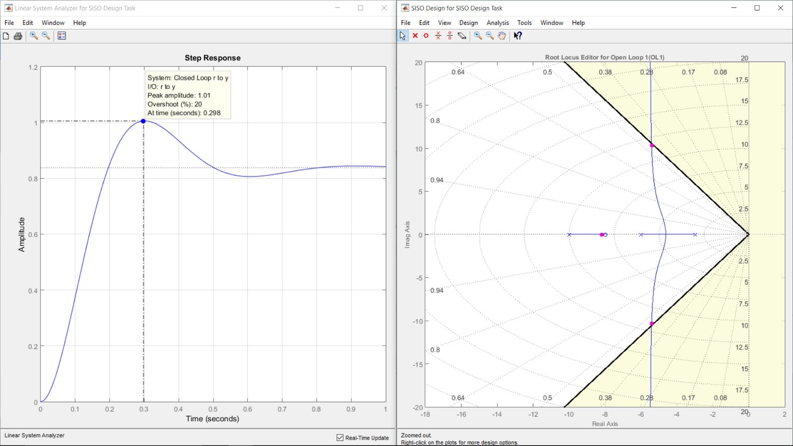 Figure 2 - The uncompensated system will have to reach a gain of about 116.5 in order to achieve the 20% overshoot (the only design characteristic at this point)
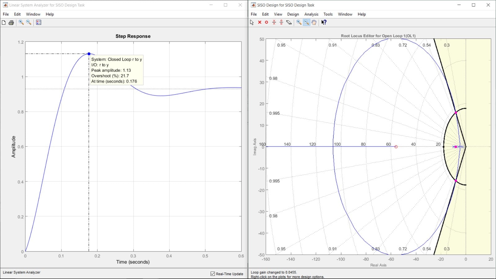 Figure 3 - Note that the borders of the two design requirements meet at certain point. Altering the gain will cause that point will position the poles.. Placing the zero at -56 will provide the plot to cross over the junction point, then adjust its gain.
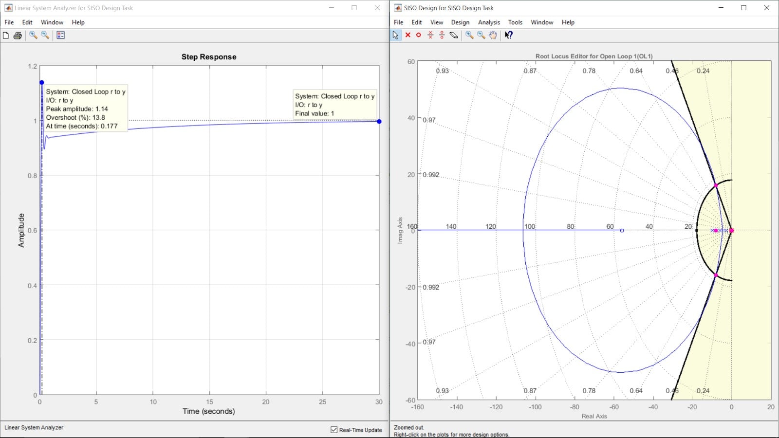 Figure 4 - The goal is to design an ideal integrator that will bring the steady-state error to zero. This is achieved by placing a pole at the origin and a zero close to the origin (rule of thumb is anything less than or equal to 0.8); in this case, choose to place the zero at -0.1. Feel free to adjust these numbers and see how the system’s reaction changes.
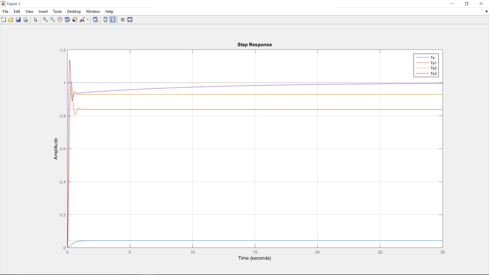 Figure 5 - This shows the step response of the given system with zero gain (for reference), uncompensated (with gain), with PD controller, and finally with PID controller
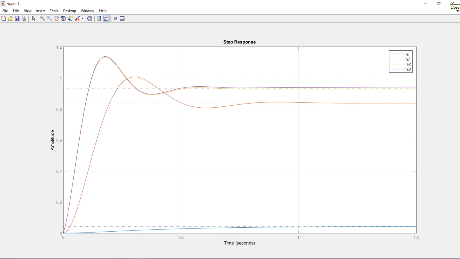
Figure 6 - A better view of our peak responses
Conclusion
As previously mentioned, this article attempted to substitute the mathematical modeling and analysis by using visual manipulations of the system’s behavior and requirements. As our end result shows, we were able to meet our design requirements and implement the mathematical model of our compensator. It’s important to note that it would require an active circuit to implement the design our PID controller, and that there are several viable solutions to our problem. Should you decide to design your own controller for the same system, it is recommended that you choose different values for the poles and zeroes.
It is likely that you could design a controller that still meets the requirements and does not have the exact values as shown above. Upon analysis of figure 5, it becomes clear how each step impacted our end result. By simply defining the region of overshoot and adjusting our gain, we were able to achieve an output that resembled our input (albeit with an obvious error). By looking at figure 6, we can immediately tell that our next attempt (PD controller) was able to dramatically improve our peak time and steady-state error. Finally, our PID was able to take what we already had defined in our PD and improve our steady-state error to our goal of zero. Becoming proficient with the SISO tool not only helps improve the time it takes to design a functional controller, but helps to ingrain the relationships of each aspect/component to our end result.
Related Content


Wow! This one article was better than my entire controls class.
I get ” Undefined function or variable ‘C’. ” when running you your code. I don’t get what this C means, and it’s really not defined in the code. MATLAB should’ve created it in some previous step?