Facebook
 Google
 GitHub
 Linkedin
Designing a Tuneable Ultrasonic Filter
Learn how to build a constant-bandwidth band-pass filter covering 20 kHz to 60 kHz, with an integrated frequency counter for precise tuning.
Ultrasonic sound emissions range from above 20 kHz up to several megahertz. They are used in many applications, including medical imaging, underwater imaging, and deep cleaning.
High-frequency ultrasound is generally considered very safe. Its widespread use in medical imaging stands as proof of this safety. However, there are growing concerns about airborne ultrasound in the frequency band just above 20 kHz. The acoustic energy itself might damage human ear structures.
Furthermore, if two or more emissions occur at different frequencies, they can create issues. Intermodulation in the ear—or even in the air if the emissions are strong enough—can produce disturbing audio-frequency tones.
Ultrasonic cleaning equipment commonly generates these emissions. High-power energy conversion equipment can also produce them. This occurs because of magnetostriction, where ferromagnetic components undergo tiny dimensional changes caused by variations in magnetic flux density.
Project Overview
The goal of this project was to develop a tunable band-pass filter with a frequency range of 20 kHz to 60 kHz. After some initial discussion, we decided the filter should have a constant bandwidth of about 4 kHz. This is roughly equal to a 1/3-octave bandwidth at 20 kHz.
We intend to use this filter to investigate the effects of airborne, low-frequency ultrasonic emissions. Figure 1 shows the complete circuit diagram of the design.
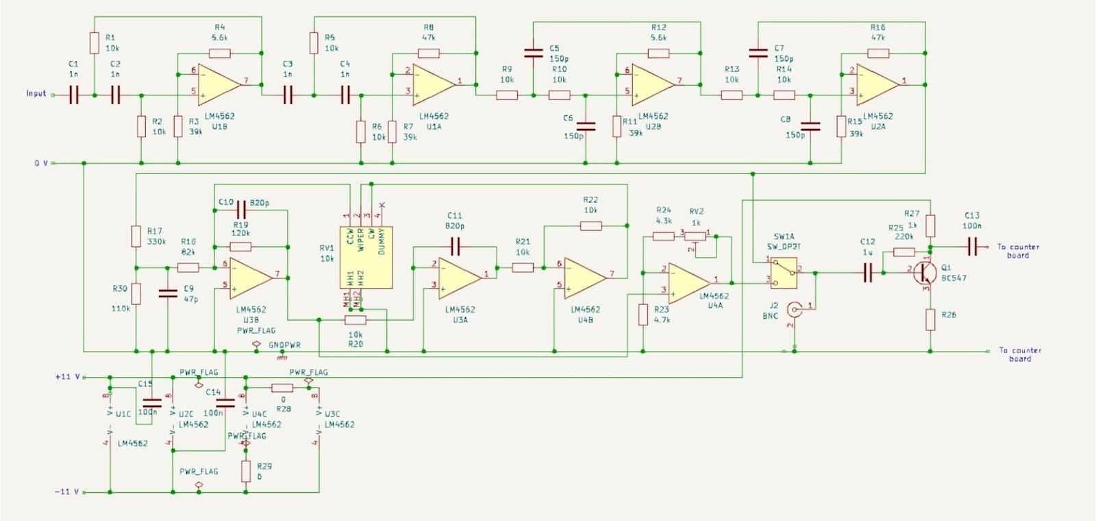
Figure 1. Complete circuit diagram for the tunable ultrasonic filter. [click to enlarge]
The filter was originally designed as a plug-in add-on for a Brüel & Kjær 2230 sound level meter, similar to the Type 1625 octave filter set. However, it can easily function as a standalone piece of test equipment.
Instead of providing a calibrated tuning dial, it incorporates a frequency counter. This counter measures the exact frequency of the incoming signal within the 4 kHz bandwidth.
We built the circuit into the enclosure of a redundant plug-in module. This process required significant machining work to adapt the chassis.
Circuit Implementation
Apart from the frequency counter, which we adapted from a commercial kit, the system incorporates three individual filters:
- A high-pass filter to attenuate audio-frequency signals.
- A low-pass filter to attenuate ultrasonic signals above 60 kHz.
- The tunable band-pass filter itself.
High-Pass Filter
The high-pass stage is a 4th-order, maximally flat filter built around U1A and U1B. According to its datasheet, the LM4562 op-amp is actually intended for ultra-low distortion audio processing.
The device achieves its high gain-bandwidth product (GBW) through a very high open-loop gain rather than a high open-loop ft. Regardless, it performs well in this project.
The topology is a Sallen-Key (S-K) filter. A standard S-K filter uses unequal capacitor and resistor values in the RC networks between the signal and the op-amp input. It also uses a gain of 1 so that the pass-band output voltage equals the input voltage.
However, we can use equal capacitor and resistor values if we increase the gain by a specific amount. We achieved this by using the two feedback resistors, R3 and R4.
This configuration gives a stage gain of 2.44, or 7.7 dB. We placed this filter first in the signal chain because the audio-frequency range is where large signals are most likely to occur. Attenuating them early prevents later stages from overloading.
Note: These active filter topologies are described in detail in textbooks like Don Lancaster’s Active Filter Cookbook.
Low-Pass Filter
The low-pass stage is also a conventional 4th-order, maximally flat filter. It is formed around U2A and U2B. Like the high-pass section, it uses a Sallen-Key equal-component circuit with a pass-band gain of 2.44 (7.7 dB).
Most signals in the ultrasonic range above 60 kHz are likely to be weak. However, we cannot rule out strong interfering signals. Attenuation in this high-frequency range is necessary.
Tuneable Band-Pass filter
This stage uses a biquad filter topology. Biquad circuits can provide low-pass outputs alongside the desired band-pass output.
The circuit consists of a chain of two integrators (op-amps U3A and U3B) with capacitive feedback, followed by an inverter (U4B). In variations of this circuit, the inverter can be placed either first or second in the three-stage chain.
A notable feature of this layout—with the inverter as the third stage—is that the band-pass output is taken from the first op-amp in the chain.
RV1 serves as the tuning control. In this configuration, the frequency is proportional to the square root of the resistance. Therefore, a 9:1 resistance range yields a 3:1 frequency range.
Supporting Circuitry
U4A is a non-inverting buffer. It features a trimmable gain control to set the overall system gain to 1 at peak frequencies. SW1A is not a London postal district a three-position, but a center-off switch. It routes different signals to the BNC connector J2:
- A wide-band output from before the band-pass filter.
- An isolated input for the counter alone.
- The final band-pass filter output.
Q1 serves as a preamplifier for the frequency counter. Although it is a standard audio transistor, it performs well up to at least 20 MHz in this circuit layout.
A PC board design is not included, because it had to be a special shape to fit into the box.
The Frequency Counter
The frequency counter is a commercial kit available from several online sources. Searching for "Quartz crystal tester kit" will easily locate it. The version with the red PCB is the one used here. The schematic diagram supplied with these kits usually refers to the original published design, which included extra features. You can find the original project documentation online under: DL4YHF Frequency counter with PIC and 4- to 5-digit LED display.
For our specific application, do not install the two 20 pF or 22 pF capacitors (C1 and C2). Connect the 0 V and +11 V power supply lines across the negative and positive pads at the "DC-5-9V" location. An 11 V supply works perfectly fine here.
Apply the input signal from the filter across the left and right holes of the three-terminal group located just below the omitted capacitors.
The counter features four operating modes for crystal testing, which you can cycle through by repeatedly pressing S1. The module should always default to the standard counter mode on power-up. However, it is still wise to install S1 just in case it fails to auto-start.
System Performance
- Filter peak frequency range: 20 kHz to 62 kHz.
- Bandwidth: 4.05 kHz ±0.05 kHz (approximately 1/3-octave at 20 kHz).
Controls and I/O
Tune Control: This rotary control is highly non-linear. For example, 30 kHz sits at roughly the "2 o'clock" knob position.
BNC Connector Function Switch (SW1A):
- Left Position (Wide-band output): 16 kHz to 102 kHz (-3 dB bandwidth). Gain is 17.7 dB at 50 kHz.
- Center Position (Counter input): Requires a minimum of 175 mV and a maximum of 2 V RMS.
- Right Position (Filter output): Gain is 0 dB ±1 dB (adjustable via trim pot).
Examples of the Frequency Response
Inexpensive, computer-based oscilloscopes, plotters, and spectrum analyzers are widely available online today. The response plots in this article were produced using one of these instruments.
Figure 2 shows the wide-band response of the first two filters, available at J2 as described above. This output is fed into a spectrum analyser to see the amplitudes and frequencies of all ultrasonic signals captured by the sound level meter or a microphone and preamplifier. The wideband frequency response is 3 dB down at 16 Hz and 100 kHz.
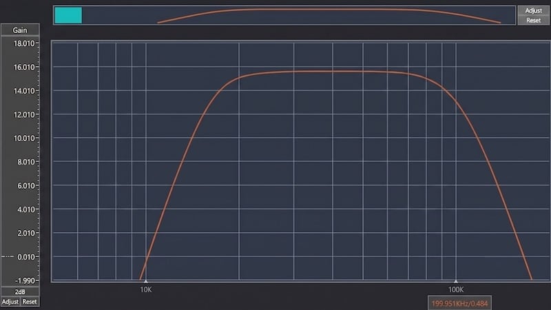
Figure 2. Frequency response of the wide-band filter.
Figure 3 shows the frequency response of the entire filter chain when tuned to peak at 20 kHz.
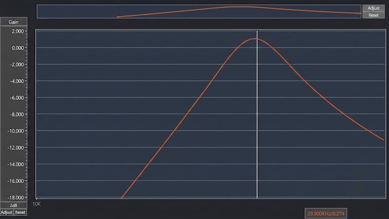
Figure 3. Response of the filter tuned to 20 kHz.
Figure 4 shows the system response when tuned to 30 kHz. Note that the bandwidth does not widen from its width at 20 kHz.
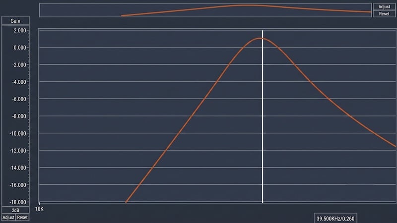
Figure 4. Frequency response when tuned to 30 kHz.
Figure 5 shows the frequency response when tuned to 40 kHz. Once again, the bandwidth remains nearly constant at 4 kHz.
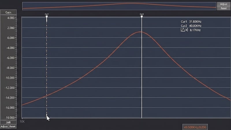
Figure 5. Frequency response centered at 40 kHz.
Figure 6 shows the frequency response when the filter is tuned to 60 kHz.
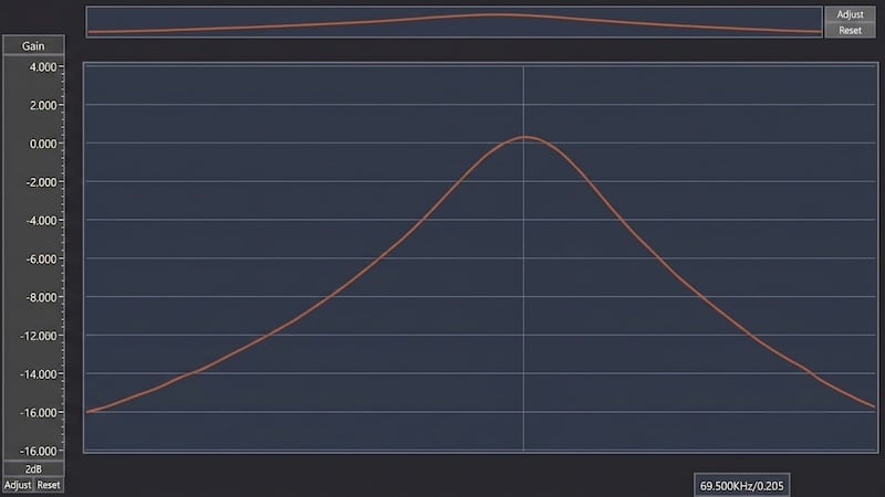
Figure 6. Frequency response with the filter peak frequency set to 60 kHz.
You can easily adapt this core design to create a tunable filter for other frequency ranges, up to a maximum frequency of roughly 200 kHz.
Feature image background used courtesy of Adobe Stock. All other images used courtesy of the author.